the Creative Commons Attribution 4.0 License.
the Creative Commons Attribution 4.0 License.
 | 21 Mar 2019
An energy balance model for paleoclimate transitions
Brady Dortmans
William F. Langford
Allan R. Willms
A new energy balance model (EBM) is presented and is used to study paleoclimate transitions. While most previous EBMs only dealt with the globally averaged climate, this new EBM has three variants: Arctic, Antarctic and tropical climates. The EBM incorporates the greenhouse warming effects of both carbon dioxide and water vapour, and also includes ice–albedo feedback and evapotranspiration. The main conclusion to be inferred from this EBM is that the climate system may possess multiple equilibrium states, both warm and frozen, which coexist mathematically. While the actual climate can exist in only one of these states at any given time, the EBM suggests that climate can undergo transitions between the states via mathematical saddle-node bifurcations. This paper proposes that such bifurcations have actually occurred in Paleoclimate transitions. The EBM is applied to the study of the Pliocene paradox, the glaciation of Antarctica and the so-called warm, equable climate problem of both the mid-Cretaceous Period and the Eocene Epoch. In all cases, the EBM is in qualitative agreement with the geological record.
- Article
(2058 KB) - Full-text XML
- Companion paper
- BibTeX
- EndNote


For approximately 75 % of the last 540 million years of the paleoclimate history of the Earth, the climate of both polar regions was mild and free of permanent ice-caps (Cronin, 2010; Crowley, 2000; Hubert et al., 2000). Today, both the North and South poles are ice-capped; however, there is overwhelming evidence that these polar ice-caps are melting. The Arctic is warming faster than any other region on Earth. The formation of the present-day Arctic and Antarctic ice-caps occurred abruptly, at widely separated times in the geological history of the Earth. This paper explores some of the underlying mechanisms and forcing factors that have caused climate transitions in the past, with a focus on transitions that were abrupt. The understanding gained here will be applied in a subsequent paper to the important problem of determining whether anthropogenic climate change may lead to an abrupt transition in the future.
We present a new two-layer energy balance model (EBM) for the climate of the Earth. General knowledge of climate and of climate change has been advanced by many studies employing simple EBMs (Budyko, 1968; Kaper and Engler, 2013; McGehee and Lehman, 2012; North et al., 1981; Payne et al., 2015; Sagan and Mullen, 1972; Sellers, 1969; Stap et al., 2017). In general, these EBMs facilitate exploration of the relationship between specific climate forcing mechanisms and the resulting climate changes. The EBM presented here includes a more accurate representation of the role of greenhouse gases in climate change than has been the case for previous EBMs. The model is based on fundamental principles of atmospheric physics, such as the Beer–Lambert law, the Stefan–Boltzmann law, the Clausius–Clapeyron equation and the ideal-gas equation. In particular, the modelling of water vapour acting as a greenhouse gas in the atmosphere, presented in Sect. 2.3.3, is more physically accurate than in previous EBMs and it shows that water vapour feedback is important in climate change. Also, ice–albedo feedback plays a central role in this EBM. The nonlinearity of this EBM leads to bistability (existence of multiple stable equilibrium states), to hysteresis (the climate state realized in the model depends on the past history) and to bifurcations (abrupt transitions from one state to another). Forcing factors that are included explicitly in the model include insolation, CO2 concentration, relative humidity, evapotranspiration, ocean heat transport and atmospheric heat transport. Other factors that may affect climate change, such as geography, precipitation, vegetation and continental drift, are not included explicitly in the EBM but are present only implicitly in so far as they affect those included factors.
During the Pliocene Epoch, 2.6–5.3 Ma, the climate of the Arctic region of Earth changed abruptly from ice-free to ice-capped. The major climate forcing factors (solar constant, orbital parameters, CO2 concentration and locations of the continents) were all very similar to today (Fedorov et al., 2006, 2010; Haywood et al., 2009; Lawrence et al., 2009; De Schepper et al., 2015). Therefore, it is difficult to explain why the early Pliocene climate was so different from that of today. That problem has been called the Pliocene paradox (Cronin, 2010; Fedorov et al., 2006, 2010). Currently, there is great interest in mid-Pliocene climate as a natural analogue of the future warmer climate expected for Earth, due to anthropogenic forcing. In recent years, significant progress has been achieved in understanding Pliocene climate, e.g. by Haywood et al. (2009); Salzmann et al. (2009); Ballantyne et al. (2010); Steph et al. (2010); von der Heydt and Dijkstra (2011); Zhang and Yan (2012); Zhang et al. (2013); Sun et al. (2013); De Schepper et al. (2013); Tan et al. (2017); Chandan and Peltier (2017, 2018) and Fletcher et al. (2018); see also references therein. This paper proposes that bistability and bifurcation may have played a fundamental role in determining the Pliocene climate.
The waning of the warm ice-free paleoclimate at the South Pole, leading eventually to abrupt glaciation of Antarctica at the Eocene–Oligocene transition (EOT) about 34 Ma, is believed to have been caused primarily by two major geological changes (although other factors played a role). One is the movement of the continent of Antarctica from the Southern Pacific Ocean to its present position over the South Pole, followed by the development of the Antarctic Circumpolar Current (ACC), thus drastically reducing ocean heat transport to the South Pole (Cronin, 2010; Scher et al., 2015). The second is the gradual draw down in CO2 concentration worldwide (DeConto et al., 2008; Goldner et al., 2014; Pagani et al., 2011). The EBM of this paper includes both CO2 concentration and ocean heat transport as explicit forcing factors. The results of this paper suggest that the abrupt glaciation of Antarctica at the EOT was the result of a bifurcation that occurred as both of these factors changed incrementally; and furthermore that both are required to explain the abrupt onset of Antarctic glaciation.
In the mid-Cretaceous Period (100 Ma) the climate of the entire Earth was much more equable than it is today. This means that, compared to today, the pole-to-Equator temperature gradient was much smaller and also the summer/winter variation in temperature at mid- to high-latitudes was much less (Barron, 1983). The differences in forcing factors between the Cretaceous Period and modern times appeared to be insufficient to explain this difference in the climates. Eric Barron called this the warm, equable Cretaceous climate problem and he explored this problem in a series of pioneering papers (Barron, 1983; Barron et al., 1981, 1995; Sloan and Barron, 1992). In a similar vein, Huber and Caballero (2011) and Sloan and Barron (1990, 1992) observed that the early Eocene (56–48 Ma) encompasses the warmest climates of the past 65 million years, yet climate modelling studies had difficulty explaining such warm and equable temperatures. Therefore, this situation was called the early Eocene warm, equable climate problem. The EBM of the present paper suggests that the mathematical mechanism of bistability provides plausible answers to both the mid-Cretaceous and the early Eocene equable climate problems. In fact, from the perspective of this simple model, these two are mathematically the same problem. Therefore, we call them collectively the warm, equable Paleoclimate problem. Recent progress in paleoclimate science has succeeded in narrowing the gap between proxy and general circulation model (GCM) estimates for the Cretaceous climate (Donnnadieu et al., 2006; Ladant and Donnadieu, 2016; O'Brien et al., 2017) and for the Eocene climate (Baatsen et al., 2018; Hutchinson et al., 2018; Lunt et al., 2016, 2017).
The principal contribution of this paper is a simple climate EBM, based on fundamental physical laws, that exhibits bistability, hysteresis and bifurcations. We propose that these three phenomena have occurred in the paleoclimate record of the Earth and they help to explain certain paleoclimate transitions and puzzles as outlined above. A key property of this EBM is that its underlying physical principles are highly nonlinear. As is well known, nonlinear equations can have multiple solutions, unlike linear equations, which can have only one unique solution (if well-posed). In our EBM, the same set of equations can have two or more coexisting stable solutions (bistability); for example, an ice-capped solution (like today's climate) and an ice-free solution (like the Cretaceous climate), even with the same values of the forcing parameters. The determination of which solution is actually realized by the planet at a given time is dependent on past history (hysteresis). Changes in forcing parameters may drive the system abruptly from one stable state to another, at so-called “tipping points”. In this paper, these tipping points are investigated mathematically, and are shown to be bifurcation points, which are investigated using mathematical bifurcation theory. Bifurcation theory tells us that the existence of bifurcation points is preserved (but the numerical values may change) under small deformations of the model equations. Thus, even though this conceptual model may not give us precise quantitative information about climate changes, qualitatively there is good reason to believe that the existence of the bifurcation points in the model will be preserved in similar more refined models and in the real world.
Previous climate models exhibiting multiple equilibrium states have indicated that bifurcations may cause abrupt climate transitions (Budyko, 1968; Sellers, 1969; North et al., 1981; Paillard, 1998; Alley et al., 2003; Rial et al., 2004; Lindsay and Zhang, 2005; Ferreira et al., 2010; Thorndike, 2012; Payne et al., 2015; Stap et al., 2017). None of these authors employ the recently developed mathematical theory of bifurcations to the extent used in this paper. Abrupt transitions in Quaternary glaciations have been studied by Ganopolski and Rahmstorf (2001); Paillard (2001a, b); Calov and Ganopolsky (2005) and Robinson et al. (2012). These glacial cycles are strongly influenced by orbital forcings, which are not within the scope of this paper. Scientists have long considered that abrupt transitions (or bifurcations) in the Atlantic Meridional Overturning Circulation (AMOC) were possible, and that this could contribute to abrupt climate change (Stommel, 1961; Rahmstorf, 1995; Ganopolski and Rahmstorf, 2001; Lenton et al., 2012). This type of change in the AMOC is sometimes called a Stommel bifurcation. However, that phenomenon is also outside the scope of the EBM of this paper, which does not include ocean geography or meridional dependence. (An extension of this EBM, to a partial differential equation (PDE) spherical shell model, is planned.)
With regard to the EOT, a variety of indicators, including the analysis of fossil plant stomata (Steinthorsdottir et al., 2016), imply that decreasing atmospheric pCO2 in the Eocene preceded the large shift in oxygen isotope records that characterize the EOT. It was hypothesized in Steinthorsdottir et al. (2016) that at the EOT, a certain threshold of pCO2 was crossed, resulting in an abrupt change of climate mode. Possible mechanisms for the threshold that they hypothesized are studied in Sect. 3.2.
Even for changes as recent as the mid-Holocene, there is a debate, for example, over whether the abrupt desertification of the Sahara is due to a bifurcation, as suggested in Claussen et al. (1999) using an Earth model of intermediate complexity (EMIC), or is a transient response of the AMOC to a sudden termination of freshwater discharge to the North Atlantic, as proposed in Liu et al. (2009), using a coupled atmosphere–ocean GCM (AOGCM). Similarly, for the glaciation of Greenland at the Pliocene–Pleistocene transition, recent work in Tan et al. (2018), using a coupled GCM–ice-sheet model, shows good agreement with proxy records without the need for bifurcations. The model of this paper does not adapt to these two situations, which are localized and away from the poles where the axis of symmetry restricts the dynamics and facilitates the analysis presented here.
Further investigation of climate changes, using a range of climate models from EBM and EMIC to GCM and AOGCM, is warranted to clarify the underlying mechanisms of abrupt climate change. Very sophisticated GCMs, which include many 3-D processes, are only able to run a few climate trajectories; while EBMs and EMICs may explore more possibilities and investigate climate transitions (tipping points) with major simplifications and with less effort. More rigorous mathematical analysis is possible on small models, which may then suggest lines of inquiry on large models. The Earth climate system is extremely complex. For best results, a hierarchy of climate models is necessary.
The energy balance model presented here is conceptual and qualitative. It contains many simplifying assumptions and is not intended to give a detailed description of the climate of the Earth with quantitative precision. It complements but does not replace more detailed GCMs. Geographically, this model is as simple as possible. It follows in a long tradition of slab models of the atmosphere. Previous slab models represented the atmosphere of the Earth as a globally averaged uniform slab at a single temperature T. The temperature T is determined in those models by a global energy balance equation of the form energy in = energy out. Such models are unable to differentiate between different climates at different latitudes; for example, if the polar climate is changing more rapidly than the tropical climate. In this new model, the forcing parameters of the slab atmosphere are chosen to represent each one of three particular latitudes: Arctic, Antarctic or tropics. Each of these regions is represented by its own slab model, with its own forcing parameters and its own surface temperature TS. In addition, each region has its own variable IA representing the intensity of the radiation re-emitted by the atmosphere. The two independent variables IA and TS are determined in each model by two energy balance equations, expressing energy balance in the atmosphere and energy balance at the surface, respectively. In this way, the different climate responses of these three regions to their respective forcings can be explored.
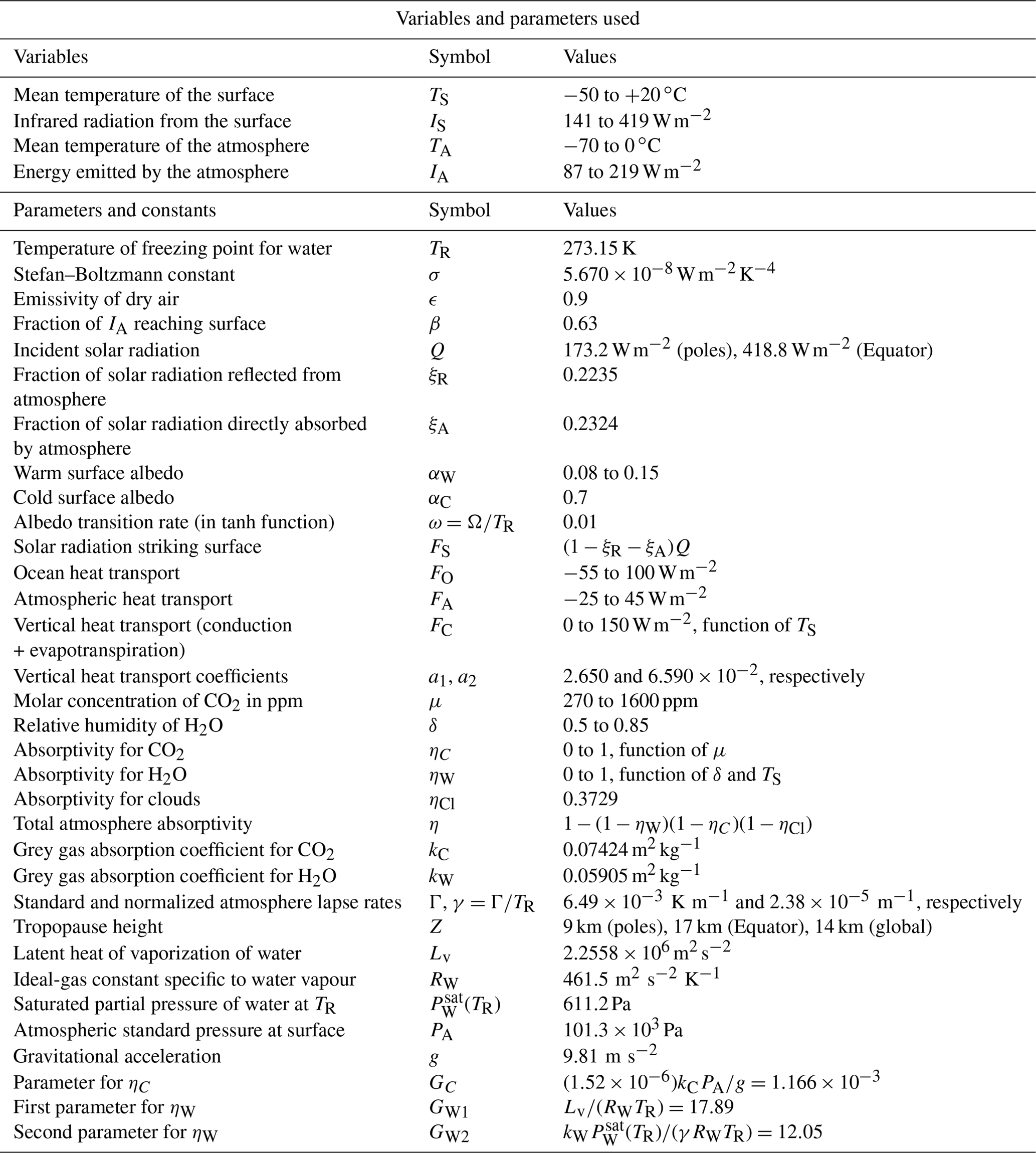
Table 1Summary of variables and parameters used in the model. Many of these parameters have standard textbook values (e.g. ). The standard lapse rate Γ is from ICAO (1993). Other parameters such as kC and kW are derived in Appendix Appendix A.
The role played by greenhouse gases in climate change is a particular focus of this model. Greenhouse gases trap heat emitted by the surface and are major contributors to global warming. The very different roles of the two principal greenhouse gases in the atmosphere, carbon dioxide and water vapour, are analyzed here in Sects. 2.3.2 and 2.3.3, respectively. The greenhouse warming effect of CO2 increases with the density of the atmosphere but is independent of temperature, while the greenhouse warming of H2O increases with temperature but is independent of the density (or partial pressure) of the other gases present. The greenhouse warming of methane (CH4) acts in a similar fashion to that of CO2; therefore, CH4 can be incorporated into the CO2 concentration. As an increase in CO2 concentration causes climate warming, this warming causes an increase in evaporation of H2O into the atmosphere, which further increases the climate warming beyond that due to CO2 alone (this is true both in the model and in the real atmosphere). This effect is known as water vapour feedback. The energy balance model presented here is the first EBM to incorporate these important roles of the greenhouse gases in such detail.
The paper concludes with two appendices. In Appendix Appendix A, model parameters that are difficult or impossible to determine for paleoclimates are calibrated using the abundant satellite and surface data available for today's climate. In addition, justification is given for parameter values chosen for the model. In Appendix Appendix B the paleoclimate model of this paper is adapted to modern-day conditions and its equilibrium climate sensitivity (ECS) is determined. Here, ECS is the change in global mean temperature produced by a doubling of CO2 in the model, starting from the pre-industrial value of 270 ppm. For this EBM, the ECS is determined to be ΔT=3.3 ∘C, which is at the high end of the range accepted by the IPCC (IPCC, 2013).
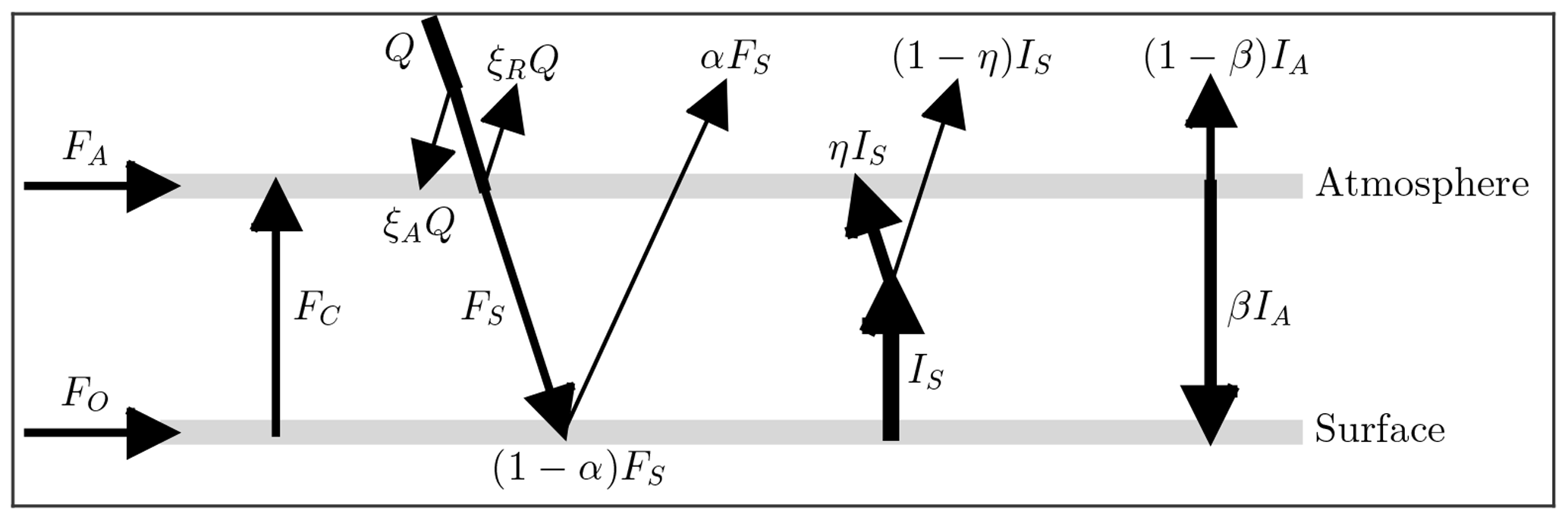
In this EBM, the atmosphere and surface are each assumed to be in energy balance. Short-wave radiant energy from the sun is partly reflected by the atmosphere back into space, a small portion is absorbed directly by the atmosphere and the remainder passes through to the surface. The surface reflects some of this short-wave energy (which is assumed to escape to space) and absorbs the rest, re-emitting long-wave radiant energy of intensity IS upward into the atmosphere. The atmosphere is modelled as a slab, with greenhouse gases, that absorbs a fraction η of the radiant energy IS from the surface. The atmosphere re-emits radiant energy of total intensity IA. Of this radiation IA, a fraction β is directed downward to the surface, and the remaining fraction (1−β) goes upward and escapes to space.
This model is based on the uniform slab EBM used in Payne et al. (2015), modified as shown in Fig. 1. In our case, the “slab” is a uniform column of air of unit cross section, extending vertically above the surface to the tropopause, and located either at a pole or at the Equator. The symbols in Fig. 1 are defined in Table 1.
This section presents the mathematical derivation of the EBM. Readers interested only in the climate applications of the model may skip this section and go directly to Sect. 3. A preliminary version of this EBM was presented in a conference proceedings paper (Dortmans et al., 2018). The present model incorporates several important improvements over that model. The differences between that model and the one presented here are indicated where appropriate in the text. Furthermore, the previous paper (Dortmans et al., 2018) considered only the application of the model to the Arctic climate and the Pliocene paradox; it did not study Antarctic or tropical climate or the Cretaceous warm, equable climate problem, as does the present paper.
2.1 Energy balance
The model consists of two energy balance equations, one for the atmosphere and one for the surface. In Fig. 1, the so-called forcings are shown as arrows, pointing in the direction of energy transfer. From Fig. 1, the energy balance equations for the atmosphere and surface are given, respectively, by
Symbols and parameter values for the model are defined in Table 1. Appendix A4 provides derivations and justification for the values of the empirical parameters. The forcings FO and FA represent ocean and atmosphere heat transport, respectively, and are specified as constants for each region of interest. Heat transport by conduction/convection from the surface to the atmosphere is denoted FC. This quantity will be largely dependent on surface temperature, TS. As described in Appendix Appendix A we have modelled it as a hyperbola that is mostly flat for temperatures below freezing, and grows roughly linearly for temperatures above freezing so that
where A1 and A2 are constants. Since the model is concerned with temperatures around the freezing point of water, we set this as a reference temperature, TR=273.15 K.
The annually averaged intensity of solar radiation striking a surface parallel to the Earth's surface but at the top of the atmosphere is Q. The value of Q at either Pole is and at the Equator is 418.8 Wm−2 (McGehee and Lehman, 2012; Kaper and Engler, 2013). A fraction ξR of this short-wave radiation is reflected by the atmosphere back into space and a further fraction ξA is directly absorbed by the atmosphere; the remainder penetrates to the surface. See Appendix A1 for the derivation of values for ξR and ξA. The solar radiation striking the surface of the Earth is
The surface albedo is the fraction, α, of this solar radiation that reflects off the surface back into space. Thus the solar forcing absorbed by the surface is (1−α)FS, and the solar radiation reflected back to space is αFS. Typical values of the surface albedo α are 0.6–0.9 for snow, 0.4–0.7 for ice, 0.2 for crop land and 0.1 or less for open ocean. In this paper we introduce a smoothly varying albedo given by the hyperbolic tangent function:
where αC and αW are the albedo values for cold and warm temperatures, respectively, and the parameter Ω determines the steepness of the transition between αC and αW. See Appendix A2 for a full explanation of Eq. (3).
The emission of long-wave radiation, I, from a body is governed by the Stefan–Boltzmann law, I=ϵσT4, where ϵ is the emissivity, σ is the Stefan–Boltzmann constant, and T is temperature. The surface of the Earth acts as a black-body radiator; so for the radiation emitted from the surface ϵ=1, thus
Previous authors have postulated an idealized uniform atmospheric temperature TA for the slab model, so that the intensity of radiation emitted by the atmosphere, IA, is
The emissivity is ϵ=0.9 since the atmosphere is an imperfect black-body radiator. A uniform temperature for the atmosphere does not exist in the real world, where TA varies strongly with height, unlike TS, which has a single value. Previous two-layer EBMs have used (TS,TA) as the two independent variables in the two energy balance Eqs. (1) and (1). Here instead, we use (TS,IA) as the two independent variables, and then we formally let TA be defined by Eq. (5). The fraction of IA that reaches the surface is β=0.63; see Appendix A6.
The parameter η represents the fraction of the infrared radiation IS from the surface that is absorbed by the atmosphere and is called absorptivity. The major constituents of the atmosphere are nitrogen and oxygen and these gases do not absorb any infrared radiation. The gases that do contribute to the absorptivity η are called greenhouse gases. Chief among these are carbon dioxide and water vapour. The contribution of these two greenhouse gases to η are analyzed in Sects. 2.3.2 and 2.3.3, respectively. Although both contribute to warming of the climate, the underlying physical mechanisms of the two are very different. In general, the contribution to η from water vapour is a function of temperature. Another major contributor to absorption is the liquid and solid water in clouds. We model this portion of the absorption as constant, since we do not include any data on cloud cover variation. However, we experimented with making this portion vary with surface temperature, and the results were not qualitatively different than those presented here.
Nondimensional temperatures
We rescale temperature by the reference temperature TR=273.15 K and define new nondimensional temperatures and new parameters
After normalization, the freezing temperature of water is represented by τ=1 and the atmosphere and surface energy balance Eqs. (1)–(4) simplify to
where, from Appendix Appendix A,
The range of surface temperatures TS observed on Earth is restricted to an interval around the freezing point of water, 273.15 K, and therefore the nondimensional temperature τ lies in an interval around τ=1. In this paper, we assume , which corresponds approximately to a range in more familiar degrees Celsius of ∘C. Another reason for the upper limit on temperature is that the Clausius–Clapeyron law used in Sect. 2.3.3 fails to apply at temperatures above the boiling point of water.
2.2 Optical depth and the Beer–Lambert law
The goal of this section is to define the absorptivity parameter η in the EBM Eq. (6) (or Eq. 1) in such a way that the atmosphere in the uniform slab model will absorb the same fraction η of the long-wave radiation IS from the surface as does the real nonuniform atmosphere of the Earth. This absorption is due primarily to water vapour, carbon dioxide and clouds. Previous energy balance models have assigned a constant value to η, often determined by climate data. In the present EBM, η is not constant but is a function of other more fundamental physical quantities, such as and T. This function is determined by classical physical laws. In this way, the present EBM adjusts automatically to changes in these physical quantities, and represents a major advance over previous EBMs.
The Beer–Lambert law states that when a beam of radiation (or light) enters a sample of absorbing material, the absorption of radiation at any point z is proportional to the intensity of the radiation I(z) and also to the concentration or density of the absorber ρ(z). This bilinearity fails to hold at very high intensity of radiation or high density of absorber, neither of which is the case in the Earth's atmosphere. Whether this law is applied to the uniform slab model or to the nonuniform real atmosphere, it yields the same differential equation
where k (m2 kg−1) is the absorption coefficient of the material, ρ (kg m−3) is the density of the absorbing substance such as CO2 and z (m) is distance along the path. The differential Eq. (6) may be integrated from z=0 (the surface) to z=Z (the tropopause) to give
Here IT≡I(Z) is the intensity of radiation escaping to space at the tropopause z=Z, and λ is the so-called optical depth of the material. Note that λ is dimensionless. The absorptivity parameter η in Eqs. (1) and (6) represents the fraction of the outgoing radiation IS from the surface that is absorbed by the atmosphere (not to be confused with the absorption coefficient k). It follows from the Beer–Lambert law that η is completely determined by the corresponding optical depth parameter λ; that is
For a mixture of n attenuating materials, with densities ρi, absorption coefficients ki and corresponding optical depths λi, the Beer–Lambert law extends to
so that
where . Equation (10) is the key to solving the problem posed in the first sentence of this subsection. For the ith absorbing material in the slab model, we set its optical depth λi to be equal to the value of the optical depth that this gas has in the Earth's atmosphere as given by Eq. (7), and then combine them using Eq. (9). This calculation is presented for the case of CO2 in Sect. 2.3.2 and for water vapour in Sect. (2.3.3). For the third absorbing material in our model, clouds, we assume a constant value ηCl.
2.3 Greenhouse gases
The two principal greenhouse gases are carbon dioxide (CO2) and water vapour (H2O). Because they act in different ways, we determine the absorptivities ηC and ηW, and optical depths λC and λW of CO2 and H2O separately, and then combine their effects, along with the absorption due to clouds, ηCl, using the Beer–Lambert law for mixtures, Eq. (10). Methane acts similarly to CO2 and can be included in the optical depth for CO2. Other greenhouse gases have only minor influence and are ignored in this paper.
2.3.1 The grey gas approximation
Although it is well-known that gases like CO2 and H2O absorb infrared radiation IS only at specific wavelengths (spectral lines), in this paper the grey gas approximation is used; that is, the absorption coefficient kC or kW is given as a single number averaged over the infrared spectrum (Pierrehumbert, 2010). The thesis by Dortmans (2017) presents a survey of values in the literature for the absorption coefficients kC and kW of CO2 and H2O, respectively, in the grey gas approximation. The values used in this paper are given in Table 1; and are derived as described in Appendix A5.
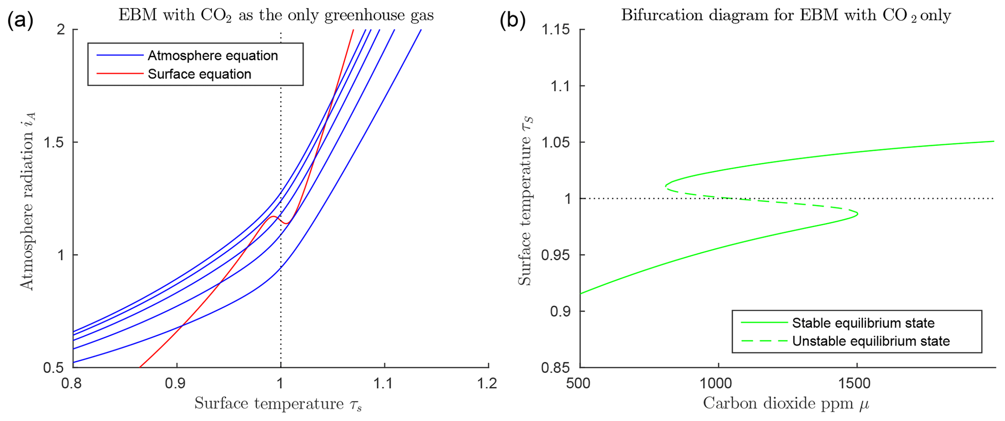
Figure 2Dry atmosphere EBM Eqs. (15)–(15) (with , , , αW=0.08 and Z=9 km). (a) CO2 values μ=400, 800, 1200, 1600, 2000; from bottom to top blue curves. A unique cold equilibrium exists for μ=400 (bottom blue curve), multiple equilibria exist for μ=800, 1200 and 1600, a unique warm equilibrium exists for μ=2000 (top blue curve). (b) Bifurcation diagram for the same parameters as in (a) showing the result of solving the EBM for τS as a function of the forcing parameter μ, holding all other forcing parameters constant. Two saddle-node (or fold) bifurcations occur at approximately μ=681 and μ=1881. Three distinct solutions exist between these two values of μ. As μ decreases from right to left in this figure, if the surface temperature starts in the warm state (τS>1), then it abruptly “falls” from the warm state to the frozen state when the left bifurcation point is reached. Similarly, starting on the frozen state (τS<1), if μ increases sufficiently, then the state will jump upward to the warm branch when the right bifurcation point is reached. Both of these transitions are irreversible (one way).
2.3.2 Carbon dioxide
The concentration of CO2 in the atmosphere is usually expressed as a ratio, in molar parts per million (ppm) of CO2 to dry air, and written as μ. There is convincing evidence that μ has varied greatly in the geological history of the Earth, and has decreased slowly over the past 100 million years; however, today μ is increasing due to human activity. The value before the industrial revolution was μ=270 ppm, but today μ is slightly above 400 ppm.
Although traditionally μ is measured as a ratio of molar concentrations, in practice both the density ρ and the absorption coefficient k are expressed in mass units of kilograms. Therefore, before proceeding, μ must be converted from a molar ratio to a ratio of masses in units of kilograms. The mass of one mole of CO2 is approximately kg mol−1. The dry atmosphere is a mixture of 78 % nitrogen, 21 % oxygen and 0.9 % argon, with molar masses of 28, 32 and 40 g mol−1, respectively. Neglecting other trace gases in the atmosphere, a weighted average gives the molar mass of the dry atmosphere as mm kg mol−1. Therefore, the CO2 concentration μ measured in molar ppm is converted to mass concentration in kg ppm by multiplication by the ratio mm. If ρA(z) is the density of the atmosphere at altitude z in kg m−3, then the mass density of CO2 at the same altitude, with molar concentration μ ppm, is
It is known that CO2 disperses rapidly throughout the Earth's atmosphere, so that its concentration μ may be assumed independent of location and altitude (IPCC, 2013). As the density of the atmosphere decreases with altitude, the density of CO2 decreases at exactly the same rate, according to Eq. (11). Substituting Eq. (11) into Eq. (7) determines the optical depth λC of CO2
Now consider a vertical column of air, of unit cross section, from surface to tropopause. The integral in Eq. (12) is precisely the total mass of this column. The atmospheric pressure at the surface is PA, and this is the total weight of the column. Therefore , where g is acceleration due to gravity. Therefore, the optical depth λC of CO2 in the actual atmosphere in Eq. (12) is
With λC so determined, it follows from Eq. (8) that
As listed in Table 1 and derived in Appendix A5, the calibrated value for kC is 0.07424, and therefore the value for the greenhouse gas parameter for CO2 is .
The dry atmosphere EBM is obtained by assuming there is no water vapour and no clouds in the atmosphere. Hence η=ηC and We assume also that . Making these substitutions in the EBM Eqs. (6)–(6) yields
Due to the nonlinearity of the ice–albedo function in 3, there can be in fact up to three points of intersection as shown in Fig. 2a. If the CO2 level μ decreases sufficiently, the warm state (τS>1) disappears, while as CO2 increases, the frozen state (τS<1) may disappear. The CO2 level μ is quite elevated in Fig. 2, but the effects of water vapour as a greenhouse gas and of clouds have been ignored.
Figure 2b introduces a bifurcation diagram (Kuznetsov, 2004), in which the two EBM Eqs. (15)–(15) have been solved for the surface temperature τS, which is then plotted as a function of the parameter μ. Figure 2b shows the three distinct solutions τS of the EBM: a warm solution (τS>1), a frozen solution (τS<1), and a third solution that crosses through τS=1 and connects the other two solutions in saddle-node bifurcations (Kuznetsov, 2004). Stability analysis (Dortmans, 2017) shows that the warm and frozen solutions are stable (in a dynamical systems sense), while the third solution (denoted by a dashed line) is unstable.
2.3.3 Water vapour and the Clausius–Clapeyron equation
In this section, we determine the absorptivity of water vapour as a function of temperature, ηW(τS), using fundamental physical laws including the Clausius–Clapeyron equation, the ideal-gas law and the Beer–Lambert law (Pierrehumbert, 2010). We also assume the idealized lapse rate of the International Standard Atmosphere (ISA) as defined by ICAO (ICAO, 1993). Unlike CO2, the concentration of water vapour (H2O) in the atmosphere varies widely with location and altitude. This is because the partial pressure of H2O varies strongly with the local temperature. In fact, it is bounded by a maximum saturated value, which itself is a nonlinear function of temperature, . The actual partial pressure of water vapour is then a fraction, δ, of this saturated value,
where δ is called relative humidity. While varies greatly with T in the atmosphere, the relative humidity δ is comparatively constant. If the actual PW(T) exceeds the saturated value (i.e. δ>1), the excess water vapour condenses out of the atmosphere and falls as rain or snow.
The saturated partial pressure at temperature T is determined by the Clausius–Clapeyron equation (Pierrehumbert, 2010),
where TR is the reference temperature, here chosen to be the freezing point of water (273.15 K); Lv is the latent heat of vaporization of water and RW is the ideal-gas constant for water, see Table 1. The actual partial pressure of water vapour at relative humidity δ and temperature T is then given by combining Eqs. (15) and (16).
We may use the ideal-gas law in the form PW=ρWRWT to convert the partial pressure PW of water vapour at temperature T to mass density ρW of water vapour at that temperature. Substituting into Eqs. (15) and (16) gives
Transforming to the dimensionless temperature as in Sect. 2.1.1, this becomes
The Beer–Lambert law in Sect. 2.2 implies that the absorptivity of a greenhouse gas ηi is completely determined by its optical depth λi. For water vapour, from Eqs. (8) and (7),
Here kW is the absorption coefficient of water vapour; see Appendix A5. In order to evaluate the integral in Eq. (19), we need to know how ρW varies with height z. We have shown that ρW is a function of temperature, given by Eqs. (17) or (18). Therefore, we need an expression for the variation in temperature T with height z. Under normal conditions, the temperature T decreases with height in the troposphere. This rate of decrease is called the lapse rate Γ, and is defined as
Normally, Γ is positive and is close to constant in value from the surface to the tropopause. The International Civil Aviation Organization has defined, for reference purposes, the ISA, in which Γ is assigned the constant value (ICAO, 1993). Using this assumption, the variation in temperature with height is given as
where the normalized lapse rate is . The tropopause height Z ranges from 8 to 11 km at the poles and 16 to 18 km at the Equator, based on satellite measurements (Kishore et al., 2006). Therefore, both T(Z) and τ(Z) are positive. For this paper we will take the height to be Z=9 km at the poles and Z=17 km at the Equator.
Equation (21) may be used to change the variable of integration in Eq. (19) for the optical depth of water vapour, from z to τ. The result is
Now substitute Eq. (18) into the integral Eq. (22) and simplify to
where the greenhouse gas parameters GW1 and GW2 for water vapour are defined as
Finally, using the Beer–Lambert law, the absorptivity ηW of water vapour in Eq. (19) is determined by its optical depth, and is now a function of the surface temperature,
The definite integral in this expression is easily evaluated numerically in the process of solving the atmosphere and surface EBM equations. As given in Table 1 and derived in Appendix A5, the calibrated value of kW is 0.05905 m2 kg−1 and the greenhouse gas parameters for H2O are
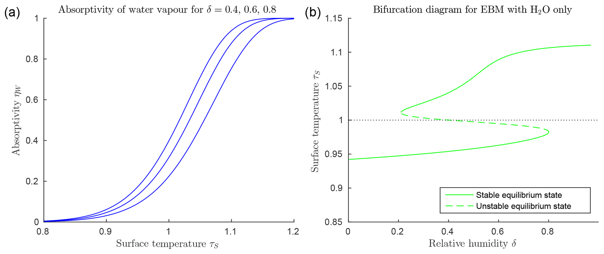
Figure 3Climate EBM (Eqs. 6–6) including greenhouse effect of water vapour only, μ=0 (with FA=45, FO=50, , αW=0.08, and Z=9 km). (a) Absorptivity ηW(τS) as given by Eq. (25) with relative humidity and 0.8 from bottom to top blue lines. Below freezing (τs<1) water vapour has little influence as a greenhouse gas, but absorptivity increases rapidly to approach η=1 for τ>1. (b) Bifurcation diagram for EBM with μ=0, and relative humidity increasing from 0 to 1. Note the accelerated increase in surface temperature τS above τS=1, compared to that in Fig. 2b, due to the rapid increase in ηW.
Figure 3a shows that the function ηW(τS) in Eq. (25) increases rapidly from near 0 to near 1 as τS increases past 1, and it steepens towards a step function as δ increases. This implies that if the surface temperature τS in the surface energy balance Eq. (6) increases past τS=1, then the absorptivity of water vapour ηW(τS), acting as a greenhouse gas in Eq. (6), increases rapidly, thus amplifying the heating of the atmosphere by the radiation from the surface. Energy balance requires a corresponding increase in the radiation IA transmitted from the atmosphere back to the surface, further increasing the surface temperature τS. This is a positive feedback loop called water vapour feedback. This positive feedback is manifested in Fig. 3b in the additional increase in TS on the warm branch, beyond that due to the ice–albedo bifurcation. Compare this with Fig. 2, where no water vapour is present. This rapid nonlinear change is due to the relatively large size of the greenhouse constant in the exponent of the Clausius–Clapeyron Eq. (18), as it reappears in Eq. (25).
2.3.4 Combined CO2 and H2O greenhouse gases
The combined effect of two greenhouse gases is determined by the Beer–Lambert law as shown in Sect. 2.2. If ηC is the absorptivity of CO2 as in Eq. (14) and ηW is the absorptivity of H2O as in Eq. (19), then the combined absorptivity η of these two is obtained by adding the two corresponding optical depths λC and λW. The overall absorptivity of the atmosphere including these two greenhouse gases and the (assumed) constant effect of clouds is, by Eq. (10),
The full nondimensional two-layer EBM is therefore specified by Eqs. (6)–(6) and (25), and the parameter values in Table 1.
2.4 Positive feedback mechanisms
The above analysis shows that there are two highly nonlinear positive feedback mechanisms in this EBM. Both serve to amplify an increase (or decrease) in surface temperature TS near the freezing point as follows. Consider the case of rising temperature. The first feedback is ice–albedo feedback, due to a change in albedo in the surface equilibrium equation. As illustrated in Fig. A1, if the surface temperature increases slowly through the freezing point, causing a drop in albedo, there is a large increase in solar energy absorbed, leading to an abrupt increase in temperature. The second is water vapour feedback in the atmosphere equilibrium equation. As shown in Fig. 3, if the surface temperature continues to increase above freezing, then the absorptivity of water vapour increases dramatically, strengthening the greenhouse effect for water vapour and further increasing the temperature. Both of these mechanisms act independently of the concentration of CO2 itself in the atmosphere. However, if the concentration of CO2 goes up, causing a rise in temperature, then each of these two positive feedback mechanisms can amplify the increase in temperature that would occur due to CO2 alone.
The goal of this section is an exploration of the underlying causes of abrupt climate changes that have occurred on Earth in the past 100 million years, using, as a tool, the EBM developed in Sect. 2. The most dramatic climate changes occurred in the two polar regions of the Earth. The climate of the tropical region of the Earth has changed relatively little in the past 100 million years. In this section, the EBMs for the two polar regions are applied to the Arctic Pliocene paradox, the glaciation of Antarctica, the warm, equable Cretaceous problem and the warm, equable Eocene problem. For comparison, a control EBM with parameter values set to those of the tropics shows no abrupt climate changes in the tropical climate for the past 100 million years.
3.1 EBM for the Pliocene paradox
The Arctic region of the Earth's surface has had ice cover year-round for only the past few million years. For at least 100 million years prior to about 3 Ma, the Arctic had no permanent ice cover, although there could have been seasonal snow in the winter. Recently, investigators have found plant and animal remains, in particular on the farthest northern islands of the Canadian Arctic Archipelago, which demonstrate that there was a wet temperate rainforest there for millions of years, similar to that now present on the Pacific Northwest coast of North America (Basinger et al., 1994; Greenwood et al., 2010; Struzik, 2015; West et al., 2015; Wolfe et al., 2017). The relative humidity has been estimated at 67 % (Jahren and Sternberg, 2003), and this value has been chosen for δ in the Arctic EBM of this section. The change from an ice-free to an ice-covered condition in the Arctic occurred abruptly, during the late Pliocene and early Pleistocene. This is sometimes called the Pliocene–Pleistocene transition (PPT 3.0–2.5 Ma; Willeit et al., 2015; Tan et al., 2018). It has been a longstanding challenge to explain this dramatic change in the climate; however, significant progress has been made recently for the case of the Greenland ice sheet (GIS). The authors of Willeit et al. (2015) have solved the “inverse problem” for the GIS by finding a schematic pCO2 concentration scenario from an ensemble of transient simulations using an EMIC that gives the best fit to data from 3.2 to 2.4 Ma, taking into account the obliquity cycle. Meanwhile, Tan et al. (2018) have used an AOGCM asynchronously coupled with sophisticated ice sheet models to reproduce the waxing and waning of the GIS across the PPT, obtaining good qualitative agreement with ice rafted debris data reconstructions.
Currently, there is great interest in the mid-Pliocene climate, because it is the most recent paleoclimate that resembles the future warmer climate now predicted for the Earth. Significant progress in understanding the Pliocene climate has been achieved in recent years. The Pliocene Research, Interpretation and Synoptic Mapping (PRISM) project of the US Geological Survey has contributed to this goal (Dowsett et al., 2011, 2013, 2016), as has the Pliocene Model Intercomparison Project (PlioMIP; Haywood et al., 2011, 2016; Zhang et al., 2013). Advances in the extraction and interpretation of proxy data have given a clearer picture of the warm Pliocene climate (Haywood et al., 2009; Salzmann et al., 2009; Ballantyne et al., 2010; Steph et al., 2010; Seki et al., 2010; Bartoli et al., 2011; De Schepper et al., 2013; Knies et al., 2014; O'Brien et al., 2014; Brierley et al., 2015; Fletcher et al., 2018). At the same time, computer models have achieved closer agreement with proxy data, see for example Haywood et al. (2009); Dowsett et al. (2011); Zhang and Yan (2012); Sun et al. (2013); Willeit et al. (2015); Tan et al. (2017, 2018); Chandan and Peltier (2017, 2018), and other references therein. Using a fully coupled atmosphere–ocean GCM, Lunt et al. (2008) considered the following forcing factors contributing to late Pliocene glaciation: decreasing carbon dioxide concentration, closure of the Panama seaway, end of a permanent El Niño state, tectonic uplift and changing orbital parameters. They concluded that falling CO2 levels were primarily responsible for the formation of the Greenland ice sheet in the late Pliocene. Recently, Tan et al. (2018) have strengthened this conclusion.
During the Pliocene Epoch, important forcing factors that determine climate were very similar to those of today. The Earth orbital parameters, the CO2 concentration, solar radiation intensity, position of the continents, ocean currents and atmospheric circulation all had values close to the values they have today. Yet, in the early/mid-Pliocene, 3.5–5 million years ago, the Arctic climate was much milder than that of today. Arctic surface temperatures were 8–19 ∘C warmer than today and global sea levels were 15–20 m higher than today, and yet CO2 levels are estimated to have been 340–400 ppm, about the same as 20th century values (Ballantyne et al., 2010; Csank et al., 2011; Tedford and Harington, 2003). As mentioned in the Introduction section, the problem of explaining how such dramatically different climates could exist with such similar forcing parameter values has been called the Pliocene paradox (Cronin, 2010; Fedorov et al., 2006, 2010; Zhang and Yan, 2012).
Another interesting fact concerning polar glaciation is that although both poles have transitioned abruptly from ice-free to ice-covered conditions, they did so at very different geological times. The climate forcing conditions of Earth are highly symmetric between the two hemispheres, and for most of the past 200 million years (or more) the climates of the two poles have been similar. However, there was an anomalous interval of about 30 million years, from the EOT, 34 Ma, to the early Pliocene, 4 Ma, when the Antarctic was largely ice covered but the Arctic was largely land ice free. Because CO2 disperses rapidly in the Atmosphere, its concentration μ must be the same everywhere at any given time. Therefore we seek a forcing factor other than μ to account for this 30-million-year period of broken symmetry. One obvious difference is geography. Since the Eocene, the South Pole has been land-locked in Antarctica, while the North Pole has been in the Arctic Ocean. Therefore, our two EBMs for the North Pole and South Pole have very different values for ocean heat transport FO. We will show that this difference is sufficient to account for the gap of 30 million years between the Antarctic and Arctic glaciations.
Our Pliocene Arctic EBM brackets the Pliocene Epoch between the mid-Eocene (50 Ma) and pre-industrial modern times, and it models the effects of the slow decrease in both CO2 and ocean heat transport FO in the Arctic over this long time interval. In this Arctic model, abrupt glaciation of the Arctic is inevitable, due to the existence of a bifurcation point.
During the Eocene (56–34 Ma), temperatures were much higher than today, especially in the Arctic (Greenwood et al., 2010; Wolfe et al., 2017; Huber and Caballero, 2011); also, CO2 concentration μ was higher than today. Estimates of Eocene CO2 concentration μ vary from 1000–1500 ppm (Pagani et al., 2005, 2006) to 490 ppm (Wolfe et al., 2017). For this EBM, we set mid-Eocene CO2 at μ=1000 (Pagani et al., 2005). Both temperature and CO2 concentration have decreased steadily but not monotonically, with many fluctuations from their Eocene values to pre-industrial modern values. The overall decrease in CO2 concentration observed since the Eocene may be attributed to decreased volcanic activity, increased absorption and sequestration by vegetation and the oceans, continental erosion, and other sinks.
The changes in ocean heat transport to the Arctic are more complicated and derive from many factors only summarized here (De Schepper et al., 2015; Haug et al., 2004; Knies et al., 2014; Lunt et al., 2008; Zhang et al., 2013). There was a slow drop in global sea level, in large part due to the gradual accumulation of vast amounts of water in the form of ice and snow on Antarctica. It has been estimated that the total amount of ice today in the Antarctic is equivalent to a change in sea level of about 58 m (Fretwell et al., 2013; IPCC, 2013). This drop in sea level likely reduced the flow of warm tropical ocean water into the Arctic. Against this background, several other factors came into play due to changing geography. In the Eocene, the North Atlantic Ocean was not always connected to the Arctic, but the Turgai Sea existed between Europe and Asia and connected the warm Indian Ocean to the Arctic, until about 29 Ma (Briggs, 1987). By the Oligocene, the Turgai Sea had closed and the North Atlantic had opened between Greenland and Norway, forming a deep-water connection to the Arctic Ocean. The Bering Strait opened and closed. During the Pliocene the formation of the Isthmus of Panama about 3.5 Ma cut off a warm equatorial current that had existed between the Atlantic and Pacific, at least since Cretaceous times. On the Atlantic side of the isthmus, the sea water became warmer, and became more saline due to evaporation. The Gulf Stream carried this warm salty water to western Europe. One might expect the Gulf Stream to transport more heat into the Arctic. However, some believe that the Gulf Stream actually contributed to glaciation in the Arctic (Haug et al., 2004; Bartoli et al., 2005) as follows. Evaporation from the Gulf Stream waters contributed to rainfall across northern Europe and Siberia, increasing the flow of fresh water in rivers emptying into the Arctic Ocean. This reduced the salinity, and hence the density, of the Arctic Ocean waters. The Gulf Stream waters in the North Atlantic now cooler, and denser due to high salinity, were forced downward by the less dense Arctic waters, which began to flow into the North Atlantic on the surface. The denser Gulf Stream waters returned southward as a deep ocean current, without having conveyed much heat to the Arctic. Meanwhile the low salinity Arctic surface water, with a higher freezing temperature, began to freeze, resulting in higher albedo and accelerating Arctic glaciation. In large measure, these changing geographical factors partially cancelled each other in their contributions to ocean heat transport to the Arctic. In the EBM, we summarize all of the above heat transport mechanisms by specifying a slow overall decrease in ocean heat transport to the Arctic, represented by the single forcing parameter FO.
Figure 4a shows graphs of the surface and atmosphere equilibrium equations for the Arctic Pliocene EBM, for varying values of μ. The figure shows only one surface equilibrium curve (red), with , because the change in FO is relatively small. The blue atmosphere equilibrium curves represent values of CO2 concentration μ falling from 1100 to 200 ppm, from the top to bottom blue curves. It is clear that there may exist up to three points of intersection of a given atmosphere equilibrium curve (blue) with the surface equilibrium curve (red); namely, a warm equilibrium state τs>1, a frozen equilibrium state τS<1 and a third (intermediate) solution, which is always unstable (when it exists). As μ decreases and the warm equilibrium state τs>1 approaches the local minimum on the red S-shaped curve, the unstable intermediate equilibrium state moves down the middle branch of the red S-shaped curve. When they meet, these two equilibria coalesce, then disappear, via a saddle-node bifurcation. Beyond this saddle-node bifurcation, only one equilibrium state remains, which is the stable frozen state on the left in the Figure. Dynamical systems theory tells us that following this bifurcation, the system will transition rapidly to that frozen equilibrium state. The paleoclimate record shows that CO2 concentration was trending downward for millions of years before and during the Pliocene. Therefore, Fig. 4a predicts that an abrupt drop in temperature to a frozen state would be inevitable if this trend continued far enough.
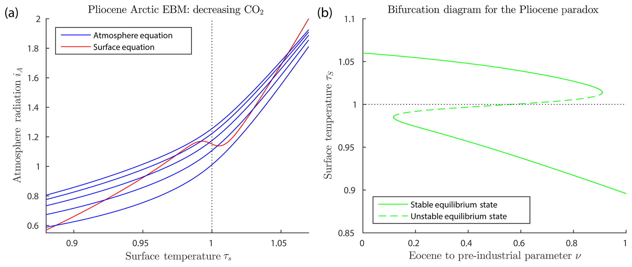
Figure 4Pliocene Arctic EBM Eqs. (6)–(6). Parameter values δ=0.67, , , αW=0.08 and Z=9 km. (a) CO2 takes values μ=200, 500, 800, 1100 and 1400 ppm from bottom to top on the blue curves with fixed on the red curve. The warm equilibrium state τS>1 disappears as μ decreases on successively lower blue curves. (b) Bifurcation diagram for the Pliocene paradox. Here, CO2 concentration μ and ocean heat transport FO decrease simultaneously with increasing ν, (), as given by Eq. (26). As ν increases, the warm equilibrium solution (τS>1) disappears in a saddle-node bifurcation at approximately ν=0.91, corresponding to forcing parameters μ=336 ppm and FO=50.9. The equilibrium temperatures at this value of ν are 3.9 and −26 ∘C, and geological time about 4.5 Ma. To the right of this point, only the frozen equilibrium state exists. Between about ν=0.12 and ν=0.91, the frozen and warm equilibrium states coexist, separated by the unstable intermediate state.
In order to explore this downward trend further, we bracket the Pliocene Epoch between the mid-Eocene Epoch (50 Ma) and the pre-industrial modern era (300 years ago), and define a surrogate time variable ν by
As reviewed above, it is believed that ocean heat transport FO decreased modestly over this time period, mainly due to the drop in global sea level, while the CO2 concentration μ decreased more significantly. Therefore, we express both μ and FO as decreasing functions of bifurcation parameter ν
Here, ν=0 corresponds to estimated mid-Eocene values of μ and FO (Pagani et al., 2005; Wolfe et al., 2017; Barron et al., 1981), while ν=1 corresponds to modern pre-industrial values (IPCC, 2013). Equation (26) defines μ and FO as linear functions of ν. In the real world, neither μ nor FO decreased linearly. This is not an obstacle for our bifurcation analysis. What is important is that, somewhere between ν=0 and ν=1, a bifurcation point is crossed.
Figure 4b is a bifurcation diagram, which shows the dependence of surface temperature τS on this bifurcation parameter ν. Note that for ν=0 (mid-Eocene values, 50 Ma) only the warm equilibrium state exists. At about ν=0.116 (44 Ma) both warm and frozen equilibrium states exist. However, as ν increases toward ν=1, the warm equilibrium state disappears in a saddle-node (or fold) bifurcation, leaving only the frozen equilibrium state to the right of the saddle-node bifurcation. This bifurcation occurs at approximately ν=0.91, which corresponds to and μ=336, which is in good agreement with the determination (Seki et al., 2010) that the warm Pliocene pCO2 was between 330 and 400 ppm, similar to today. The temperatures of the warm state and frozen state, at the bifurcation value of ν=0.91 in the EBM, are +3.9 and −26 ∘C, respectively. The surrogate time of the bifurcation point, ν=0.91, corresponds to a geological time of t=4.5 Ma, from Eq. (25), which is close to the time of glaciation of the Arctic in the geological record.
The EBM plotted in Fig. 4 provides a plausible explanation for the Pliocene paradox. For millions of years up to the mid-Pliocene, while the Arctic temperature remained above freezing on the warm solution branch in Fig. 4b, the climate change was incremental. Then the slowly acting physical forcings of decreasing CO2 concentration and decreasing ocean heat transport, FO, were amplified by the mechanisms of ice–albedo feedback and water vapour feedback, both of which act very strongly when the temperature crosses the freezing point of water. The EBM suggests that when the freezing temperature was approached, the Arctic climate changed abruptly via a saddle-node bifurcation as in Fig. 4b, from a warm state to a frozen state.
Permanent El Niño
Another explanation has been proposed for the Pliocene paradox. There is convincing evidence that at the beginning of the Pliocene, there was a permanent El Niño condition in the tropical Pacific Ocean (Fedorov et al., 2006, 2010; Steph et al., 2010; Cronin, 2010; von der Heydt and Dijkstra, 2011). However, some have disputed this finding (Watanabe et al., 2011). It has been suggested that a permanent El Niño condition could explain the warm early Pliocene, and that the onset of the El Niño–Southern Oscillation (ENSO) was the cause of sudden cooling of the Arctic during the Pliocene. Today, it is known that ENSO can influence weather patterns as far away as the Arctic. However, the present authors propose that bistability and bifurcation provide a more satisfactory explanation for the Pliocene paradox, and suggest that the concurrent change in ENSO may have been a consequence, not the cause, of the changing Pliocene Arctic climate (work in progress).
3.2 EBM for the glaciation of Antarctica
Antarctica in the mid-Cretaceous Period was ice free, and it remained so for the remainder of the Cretaceous Period and into the Paleocene and early Eocene. However, recent investigations in paleoclimate science have shown that there was an abrupt drop in temperature and an onset of glaciation in Antarctica at the EOT about 34 Ma (Katz et al., 2008; Lear et al., 2008; Miller et al., 2008; Scher et al., 2011, 2015; Ladant et al., 2014; Ruddiman, 2014). In the mid-Cretaceous, the continent of Antarctica was in the South Pacific Ocean and the South Pole was located in open ocean, warmed by South Pacific Ocean currents (Cronin, 2010). Then, the continent of Antarctica moved poleward and began to encroach upon the South Pole towards the end of the Cretaceous, fully covering the South Pole before the end of the Eocene (Briggs, 1987). The diminishing marine influence on the South Pole coincided with the onset of cooling of Antarctica about 45 Ma (mid-Eocene). The opening of both the Drake Passage (between South America and Antarctica) and of the Tasmanian Gateway (between Antarctica and Australia) near the end of the Eocene (34 Ma) led to the development of the ACC, which further isolated the South Pole from warm ocean heat transport and accelerated the cooling and glaciation of Antarctica (Cronin, 2010). Therefore, from the early Eocene to the Oligocene, the ocean heat transport to the South Polar region decreased significantly, from near the Cretaceous value, about 100 Wm−2 (Barron et al., 1981), to a much lower value, estimated here to be 30 Wm−2. The fact that the glaciation of the Antarctic took place 30 million years before the glaciation of the Arctic is very likely due primarily to the much larger decrease in ocean heat transport that took place at the South Pole.
Because the atmosphere is well mixed, at any given time the CO2 level in the Antarctic is the same as elsewhere. For this EBM, we estimate the early Eocene global CO2 level as μ=1100 ppm, (Pagani et al., 2005, 2006; Cronin, 2010); decreasing to approximately modern levels by the end of the Oligocene, 23 Ma, that is to μ=400 ppm.
In the recent literature, there has been a discussion of whether the primary cause of the onset of Antarctic glaciation is the slow decline in CO2 concentration or the decrease in poleward ocean heat transport due to the opening of ocean gateways and the development of the ACC (DeConto et al., 2008; Goldner et al., 2014; Pagani et al., 2011; Scher et al., 2015). In fact, Ladant et al. (2014) state “The reasons for this greenhouse–icehouse transition have long been debated, mainly between the 'tectonic-oceanic' hypothesis and the CO2 hypothesis”. In the work by Scher et al. (2015), it is observed that the onset of the ACC coincided with major changes in global ocean circulation, which probably contributed to the drawdown in CO2 concentration in the atmosphere. Since both CO2 concentration and ocean heat transport FO are explicit parameters in the EBM presented here, they can be varied independently in the model to investigate which one played a primary role.
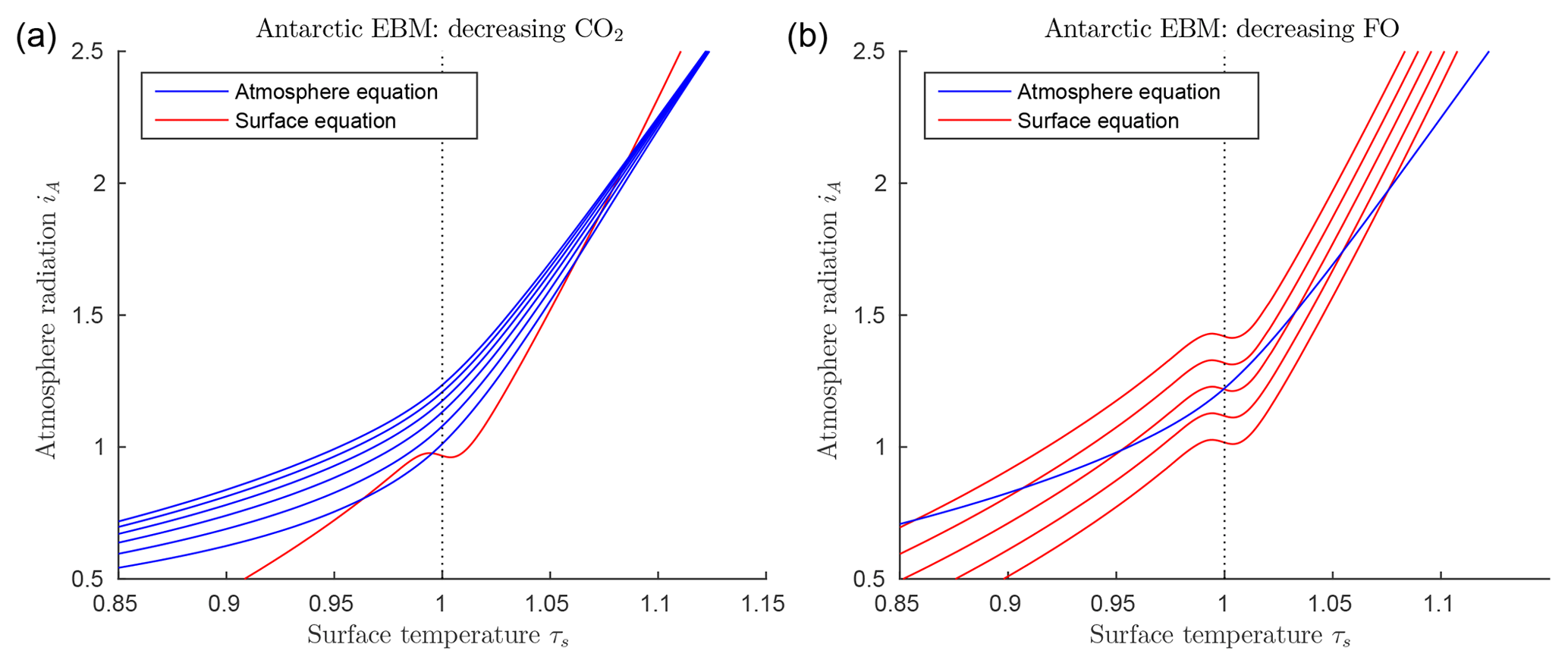
Figure 5EBM for the glaciation of Antarctica (with δ=0.67, , , αW=0.15, Z=9 km). (a) Graphs of EBM equations, with FO fixed at 90 W m−2 in the surface equation (red line), and with CO2 concentration μ in the atmosphere equation increasing (from bottom to top blue lines) and 1200 ppm. (b) Graphs of the same EBM equations but with CO2 concentration μ fixed at 1100 ppm (blue line) and with ocean heat transport FO decreasing (from bottom to top red lines) 80, 60, 40, 20 and 0 W m−2.
Figure 5 shows the solutions of the EBM equations for Antarctic parameter values, including δ=0.67, , , αW=0.15, and Z=9 km. Points of intersection of one red line (surface equation) and one blue line (atmosphere equation) are the equilibrium solutions of the system. As noted earlier, there can be up to three equilibrium solutions. In Fig. 5a the ocean heat transport FO is held fixed, while CO2 concentration μ is decreased from the top to bottom blue lines. In Fig. 5b the reverse is true; the CO2 concentration μ is held fixed while the ocean heat transport FO is decreased from bottom to top red lines. For a sufficiently small value of FO, the warm solution disappears in Fig. 5b. This occurs when the warm solution meets the unstable intermediate solution in a saddle-node bifurcation. Beyond this bifurcation, only the frozen solution (τS<1) exists. In contrast, reducing μ in Fig. 5a does not affect the existence of the warm equilibrium, only the existence of the cold equilibrium.
Figure 6 displays bifurcation diagrams in which the surface temperature τS, which has been determined as a solution of the EBM, is plotted while parameters in the EBM are varied smoothly, from the early Eocene values, 55 million years ago, to the late Oligocene values, 23 million years ago. These dates are chosen to bracket the time of the glaciation of Antarctica. First we introduce a bifurcation parameter ν, which acts as a surrogate time variable. The bifurcation parameter ν is related to geological time by
Thus, ν=0 corresponds to the early Eocene, 55 Ma, and ν=1 corresponds to the late Oligocene, 23 Ma. During this time, it is known that both CO2 concentration μ and ocean heat transport FO were decreasing. To study the effects of the simultaneous reduction of μ and FO, we express both as simple linear functions of the bifurcation parameter ν, as follows:
Here, ν=0 corresponds to the high early Eocene values of μ=1100 ppm and , while ν=1 corresponds to the low Oligocene–Miocene boundary values of μ=400 ppm and . Thus, in Eq. (27), as ν increases from 0 to 1, the climate forcing factors μ and FO decrease linearly from their Eocene values to late Oligocene values. Strictly speaking, these forcings did not change linearly in time; however, the important fact is that overall they were decreasing, For our bifurcation results the decrease does not need to be linear in the EBM. The atmospheric heat transport parameter FA is held constant at . The solar radiation is , the warm albedo value is αW=0.15 and the tropopause height is Z=9 km. Other parameters are as in Table 1.
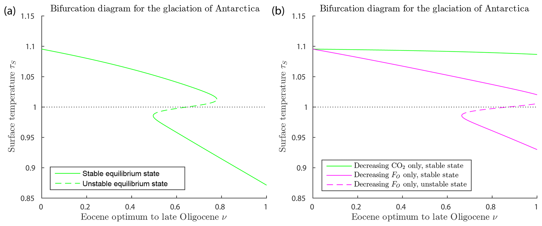
Figure 6Bifurcation diagrams for the glaciation of Antarctica (with δ=0.67, FA=45, , αW=0.15, Z=9 km). (a) This shows a saddle-node bifurcation at ν=0.779, corresponding to forcing parameter values μ=555 ppm and in Eq. (27). As ν increases through this saddle-node bifurcation point, the climate will transition abruptly from a warm state to a frozen state. The warm state and frozen state temperatures coexisting at the bifurcation point are +3.5 and −22.1 ∘C. (b) Two superimposed bifurcation diagrams as in (a), except that, on the green curve, FO is held fixed at its Eocene values while μ deceases as in Eq. (27), and, on the magenta curve, μ is held fixed at the Eocene value while FO decreases as in Eq. (27). No saddle-node bifurcation destroying the warm equilibrium occurs in either scenario.
Figure 6a shows a saddle-node bifurcation at ν=0.779, corresponding to forcing parameter values μ=555 ppm and in the model, and to geological time about 30 Ma, assuming the linear time relation in Eq. (26). This corresponds closely to best estimates of the timing of glaciation in the geological record of about 34 Ma at the EOT. This quantitative agreement should not be taken very seriously, as it is largely due to assumptions made in the modelling. However, the existence of the bifurcation, implying an abrupt glaciation of Antarctica, can be taken seriously, as this is a robust (structurally stable) property of the model. The warm state and frozen state temperatures coexisting at the bifurcation point are +3.5 and −22.1 ∘C. As ν increases past the bifurcation point ν=0.779, the warm climate state ceases to exist, and the climate system transitions (“falls”) rapidly from the saddle-node point to the frozen state. Thus the EBM reproduces the abrupt transition to the glaciation of Antarctica, which is seen in the geological record at the EOT.
Figure 6b explores the relative importance of decreasing CO2 concentration μ and decreasing ocean heat transport FO in the glaciation of Antarctica, a subject that has been much debated in the literature (DeConto et al., 2008; Goldner et al., 2014; Ladant et al., 2014; Miller et al., 2008; Pagani et al., 2011; Scher et al., 2011, 2015). The green curve represents a scenario in which μ decreases as in Eq. (27) but FO is held fixed at its Eocene value, and the magenta curve represents a case in which μ is held fixed at its Eocene value while FO decreases according to Eq. (27). In neither case does a glaciation event occur. The analysis of this paper implies that significant decreases in both CO2 concentration μ and ocean heat transport FO are required to achieve a saddle-node bifurcation, reproducing the observed transition to a frozen Antarctic state at the EOT.
While the glaciation of Antarctica is an accepted fact in paleoclimate science (Miller et al., 2008; Lear et al., 2008; Pagani et al., 2011; Scher et al., 2011; Goldner et al., 2014; Scher et al., 2015), the suddenness of the climate change that occurred in Antarctica near the Eocene–Oligocene transition (34 Ma), a time when the forcing parameters were changing slowly, has been difficult to explain. The bifurcation analysis presented here gives a simple but plausible explanation for the abruptness of this event. Furthermore, this EBM supports the hypothesis that both falling CO2 concentration μ and decreasing ocean heat transport FO (due to gateway openings and development of the ACC) are essential to an explanation of the sudden glaciation of Antarctica at the EOT.
3.3 EBM for the tropics
In the tropics, many of the values of the forcing parameters are different from their values in the Arctic and Antarctic, see Table 2. The geological record shows little change in the tropical climate over the past 100 million years, other than minor cooling. Even when the Arctic climate changed dramatically in the late Pliocene, the tropical climate changed very little.
Figure 7a shows solutions of the EBM equations for tropical parameter values. Note that at no value of the forcings used here does the warm equilibrium point approach a saddle-node bifurcation point. Thus, our EBM is in agreement with the geological record.
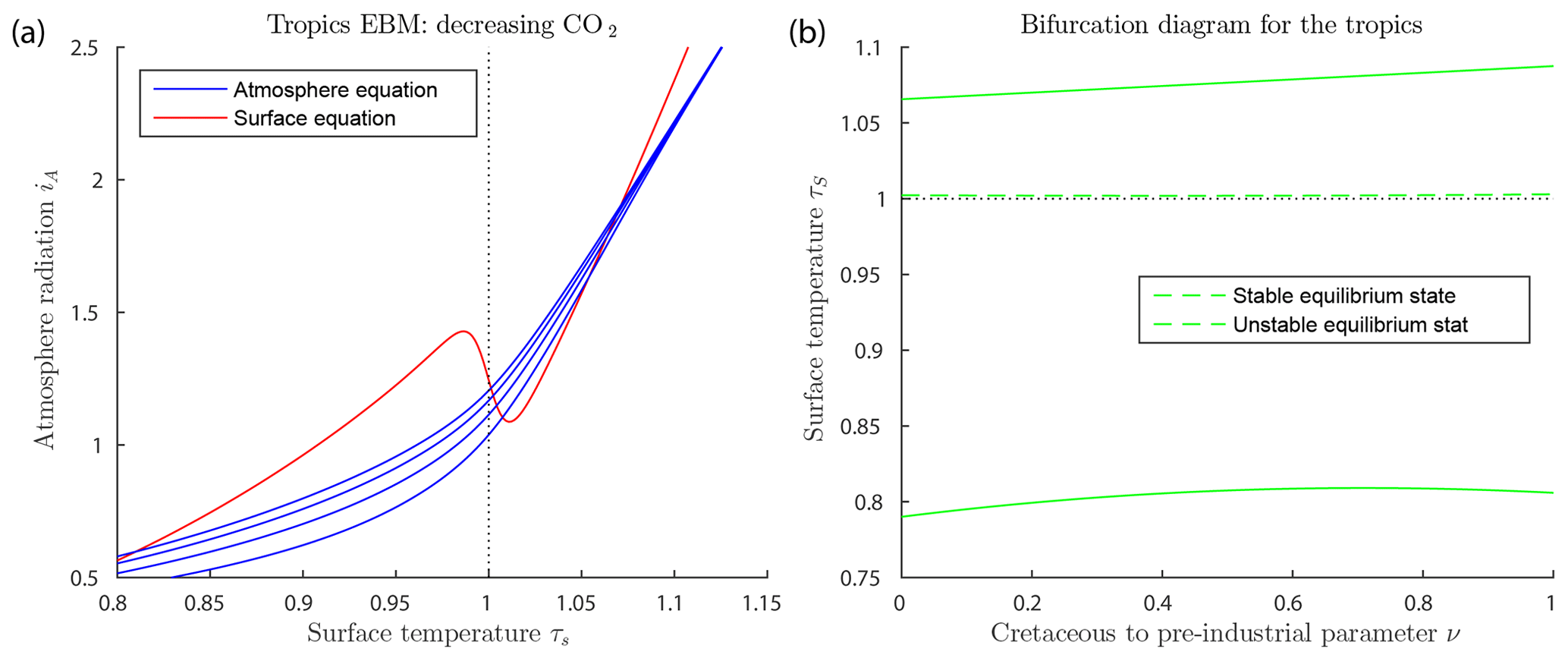
Figure 7Tropics EBM, using Eqs. (6)–(6) and parameter values as in Table 2. (a) The blue curves represent the atmosphere equilibrium equation for and 1200 from bottom to top. (b) Bifurcation diagram for the tropics EBM. Here, CO2 concentration μ and ocean heat transport FO are both decreasing, with increasing ν, (), as given by Eq. (27). As ν varies, both the warm equilibrium state (τS>1) and the frozen equilibrium state (τS<1) persist; there are no saddle-node bifurcations.
Table 2Summary of parameters used in the tropics EBM. Relative humidity δ is higher in the tropics than the Arctic, and the forcings FO and FA are negative instead of positive. The insolation Q is as determined by McGehee and Lehman (2012). Tropopause height Z is from Kishore et al. (2006). Parameters not listed here are as in Table 1.
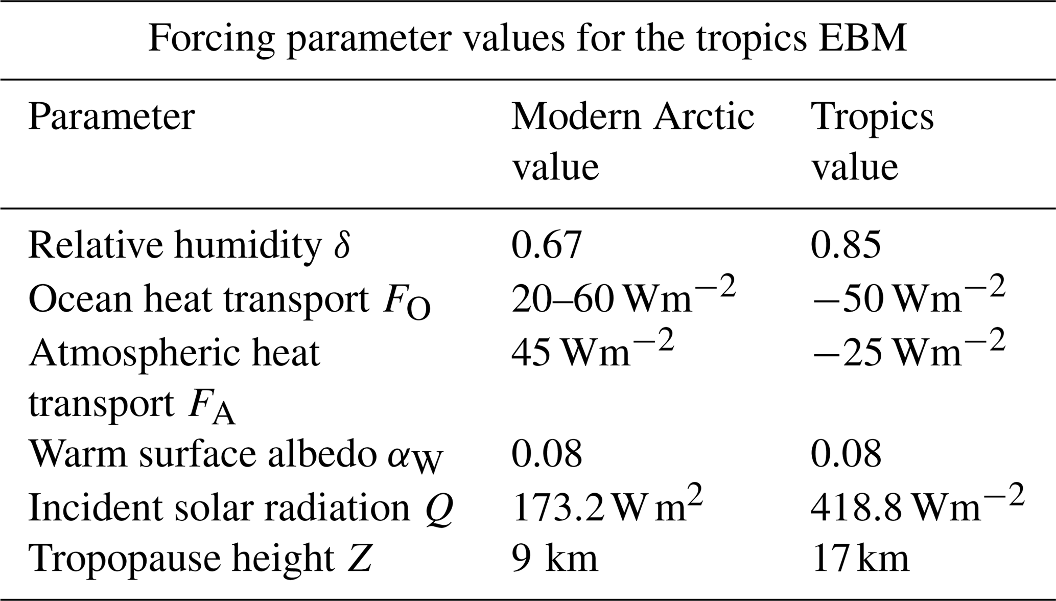
A bifurcation diagram is constructed for the tropics EBM, spanning mid-Cretaceous to modern pre-industrial times, similar to those for the Antarctic and Arctic glaciations. Here ν=0 corresponds to mid-Cretaceous values and ν=1 corresponds to modern pre-industrial values. We let μ and FO decrease linearly with ν.
The mid-Cretaceous CO2 concentration μ=1130 ppm is as determined by Fletcher et al. (2008), see Table 3. The ocean heat transport , from the tropics in the mid-Cretaceous, is from Barron et al. (1981). Astrophysicists have determined that solar luminosity is slowly increasing with time (Sagan and Mullen, 1972). For the mid-Cretaceous, insolation was approximately 1 % less than it is today (Barron, 1983). This difference is considered too small to be significant in our model. The bifurcation diagram for the tropics EBM is shown in Fig. 7b. Note that no bifurcations occur for parameter values relevant to the tropics. This is in agreement with paleoclimate records that show little change in tropical climate, even when polar climates changed dramatically.
3.4 EBM for the Cretaceous and Eocene warm, equable climate problems
One hundred million years ago, in the mid-Cretaceous Period, the climate of Earth was much more equable than today. “More equable” means that the pole-to-Equator temperature gradient was much smaller, and also the seasonal summer/winter temperature variations were much smaller. The climate in the tropics was only slightly warmer than today, but the climate at both poles was much warmer than today. An abundance of plant and animal life thrived under these conditions, from the Equator to both poles, including of course dinosaurs. The question of how this globally ice-free climate could have been maintained was explored in pioneering work of Barron and coworkers (Barron, 1983; Barron et al., 1981, 1995; Sloan and Barron, 1992). Barron called this the warm, equable Cretaceous climate problem. Early GCMs of the 1980s adjusted to mid-Cretaceous forcing parameter values, had difficulty giving good agreement with climate proxies. In order to obtain polar temperatures in agreement with mid-Cretaceous values, these simulations typically assumed increased CO2 levels more than 4 times modern levels; but then the tropical temperatures predicted by the models were too high. Today, the issue of reproducing an equable Equator-to-pole temperature gradient remains a challenge for modellers.
There have been many investigations of the correlation between early climate models and proxy data for the Cretaceous climate (Pagani et al., 2005; Bice et al., 2006; Donnnadieu et al., 2006; Cronin, 2010; Ruddiman, 2014). Recent studies have succeeded in narrowing the gap (Craggs et al., 2012; Bowman et al., 2014; O'Brien et al., 2017; Lunt et al., 2016; Ladant and Donnadieu, 2016). Based on ocean drilling samples, Bice et al. (2006) estimate Cretaceous CO2 concentrations between 600 and 2400 ppmv, and tropical Atlantic upper ocean temperatures between 33 and 42 ∘C. Based on fossil samples, Fletcher et al. (2008) estimate mid-Cretaceous atmospheric CO2 concentrations of 1130 ppmv and we choose their estimate for use in this EBM, see Table 3.
Fletcher et al. (2008)Jahren and Sternberg (2003)Barron et al. (1981)Barron et al. (1981)Table 3Summary of parameters used in the polar mid-Cretaceous model. The main difference in Cretaceous climate between the two poles was that ocean heat transport was much higher in the Antarctic. Parameters not listed here are the same as in Table 1. The values of FA and FO shown here are estimated from Barron et al. (1981).
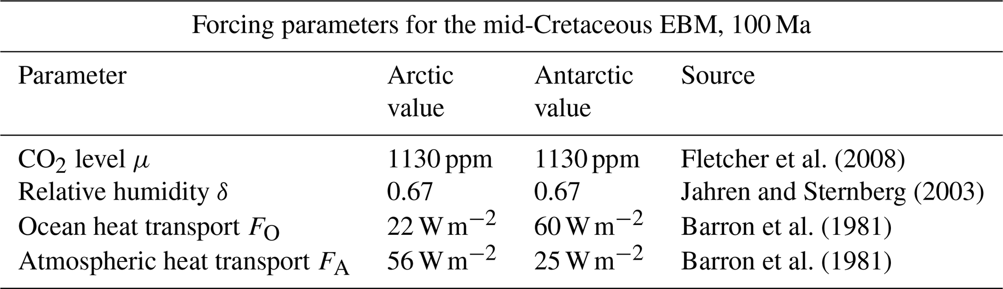
Paleoclimate data from the mid-Cretaceous show little difference in climate between the two warm poles at that time (Barron, 1983; Barron et al., 1981). The major difference in forcings between the two poles at that time was that ocean heat transport FO was much higher in the Antarctic than the Arctic, as shown in Table 3. This is due to the location of the South Pole in open ocean during the Cretaceous, as the continent of Antarctica had not yet drifted to its present position over the South Pole. Estimates for atmospheric transport are also different (Barron et al., 1981). Therefore, we model the mid-Cretaceous climate at the two poles using Eqs. (6)–(6), with the values from Table 3. The EBM equilibrium curves are shown in Fig. 8, where it is clear that a warm (τS>0) and a frozen (τS<0) equilibrium state exists at both poles for the given parameter values. The Antarctic warm equilibrium state is warmer than in the Arctic because of the higher ocean heat transport FO to the Antarctic. From Sect. 3.3, the tropical region of Earth also had a warm equilibrium state under mid-Cretaceous conditions. Therefore, the EBM of this paper implies the existence of a pole-to-pole warm, equable Cretaceous climate, as is seen in the geological record.
Figure 8 also implies that a frozen equilibrium state is mathematically possible at each pole during the Cretaceous. In that case, the tropics could remain in the warm state, thus giving the mathematical possibility of a Cretaceous climate that is not equable, but has warm tropics and ice-covered poles, like today's climate. This may help explain why some computer simulations, originally designed for today's climate conditions, found a mathematically existing Cretaceous climate that resembled today's climate more than the warm, equable climate that physically existed on Earth in the Cretaceous.
The climate of the Eocene Epoch (≈55 million years ago) was the warmest of the past 65 million years, but a little cooler than the Cretaceous (Sloan and Barron, 1992; Pagani et al., 2005; Cronin, 2010; Huber and Caballero, 2011; Hutchinson et al., 2018). Both poles were ice-free and the pole-to-Equator temperature gradient was much smaller than today. As for the mid-Cretaceous, early computer simulations, based on modern climate conditions, had difficulty in reproducing the early Eocene warm, equable climate (Sloan and Barron, 1990, 1992; Sloan and Rea, 1995; Jahren and Sternberg, 2003; Huber and Caballero, 2011). This discrepancy has been called the early Eocene warm, equable climate problem. Here we combine these two “problems” under one name as the warm, equable Paleoclimate problem.
The main difference in forcings between early Eocene conditions and those of the mid-Cretaceous is that the global CO2 concentration μ may have been a little lower and the ocean heat transport FO to the Antarctic was less. Referring to Fig. 8, this means that the blue and green atmosphere equilibrium curves move downward slightly, and the magenta Antarctic surface equilibrium curve moves upward slightly. The orange Arctic surface equilibrium curve does not change significantly. With these small changes, all of the equilibrium climate states (intersection points) persist in Fig. 8. The figure for the Eocene EBM (not shown here) is topologically the same as Fig. 8 for the mid-Cretaceous EBM,
Thus, the EBM predicts that a warm ice-free equilibrium state exists (mathematically) at both poles in the mid-Cretaceous and early Eocene. From Sect. 3.3, the equatorial region also has a warm equilibrium state for Eocene conditions. Therefore, this EBM study supports the existence of a pole-to-pole warm, equable climate in both the mid-Cretaceous and the early Eocene. Additionally, in the EBM there is the coexistence of a nonequable climate, with cold poles, under exactly the same forcing conditions, which suggests the following plausible solution to the “warm, equable paleoclimate problem” in both the mid-Cretaceous (Barron, 1983; Barron et al., 1981, 1995; Sloan and Barron, 1990) and the early Eocene (Sloan and Barron, 1990, 1992; Sloan and Rea, 1995; Jahren and Sternberg, 2003; Huber and Caballero, 2011). While the Earth's climate existed in the warm, equable climate state of the EBM, computer simulations of Barron and others may have correctly computed the coexisting nonequable solution.
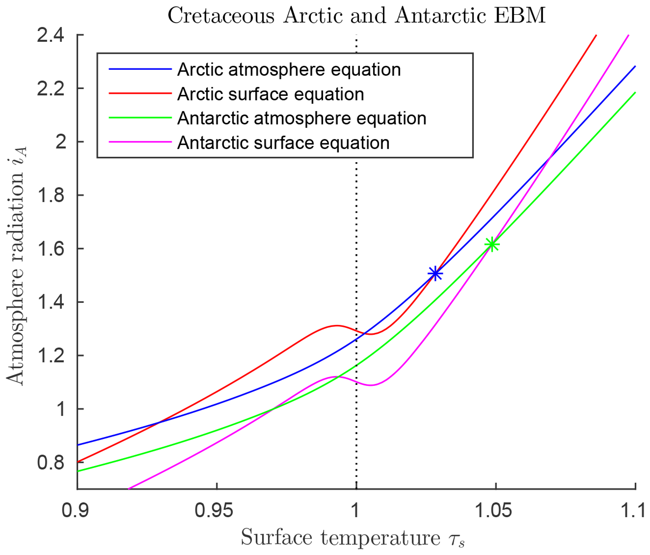
Figure 8Solutions of the mid-Cretaceous EBM for both poles, using parameter values in Table 3. The blue and orange curves represent the EBM for the Arctic while the green and magenta curves represent the Antarctic. The two Z-shaped curves represent the surface equilibrium equations for the Arctic (upper orange curve) and the Antarctic (lower magenta curve). The only differences in these two are that ocean heat transport FO is much greater in the Antarctic than the Arctic, and the atmospheric transport, FA, is smaller. Both poles support both warm and frozen equilibrium paleoclimate states. The warm equilibrium states at the two poles are marked by stars.
This paper presents a new energy balance model (EBM) for the climate of Earth, one that elucidates the distinctive roles of carbon dioxide and water vapour as greenhouse gases, and also the role of ice–albedo feedback, in climate change. Nonlinearity of the EBM leads to multiple solutions of the mathematical equations and to bifurcations that represent transitions between coexisting stable equilibrium states. This EBM sheds new light on several important problems of paleoclimate science; namely, the Pliocene paradox, the abrupt glaciation of Antarctica, and the warm, equable mid-Cretaceous and early Eocene climate problems. Predictions of the EBM are in qualitative agreement with the paleoclimate record.
There has been a range of values of paleoclimate forcing parameters in the literature, in particular for mid-Cretaceous and Eocene CO2 concentrations and temperatures. The specific choices made here, while informed by proxies, are somewhat arbitrary. However, this fact does not affect the validity of our main conclusions. The coexistence of multiple solutions and the bifurcations demonstrated in the EBM are robust phenomena. That is, the existence of these multiple solutions and bifurcations will persist over a range of values of the forcing parameters. The main conclusion of this paper that sudden and significant changes in climate have occurred, even while forcing parameters were changing very gradually, follows from the existence of mathematical bifurcations in the EBM, not from particular choices of the forcing parameters.
As the paleoclimate record becomes clearer, there is growing evidence for small but rapid fluctuations in some parameter values, including CO2 concentrations, over the geological time period studied here (Cronin, 2010; Pagani et al., 1999, 2005). The model of this paper assumes a smooth decline in CO2 concentration. However, this does not invalidate our main conclusions. The theory of “stochastic bifurcation” (Namachchivaya, 1990; Arnold et al., 1996) tells us that if stochastic noise is added parametrically to a deterministic bifurcation problem, then typically the location of the bifurcation (in terms of the bifurcation parameter) may change; but the existence of the bifurcation is preserved.
Further work on this EBM is in progress. Having demonstrated the applicability of the EBM to known paleoclimate transitions, this EBM is now being applied to anthropogenic climate change with the goal of predicting the future climate effects of continued increases in CO2 concentration.
The most significant question is whether a bifurcation is to be expected in our future. This bifurcation would lead to climate warming even stronger than that currently underway, leading possibly to a warm, equable climate, at least in the Northern Hemisphere, similar to the climate of Earth before the Pliocene.
The equilibrium climate sensitivity (ECS) of the EBM, adapted to present-day satellite data, has been calculated and is presented in Appendix Appendix B of this paper.
This scalar EBM will be generalized to a two-point boundary value problem (BVP) in the altitude variable z, using the Schwarzschild equations to replace the ICAO International Standard Atmosphere (ISA) approximation for lapse rate. That change will more accurately model the behaviour of the greenhouse gases in the atmosphere. Next, that one-dimensional EBM BVP will be incorporated into a generalization of the spherical shell PDE model of Lewis and Langford (2008) and Langford and Lewis (2009). We anticipate that this 3-D zonally symmetric Navier–Stokes Boussinesq model will confirm the fundamental predictions relating to bistability and bifurcation of the present simple EBM. Also, it will enable the study of a third positive feedback mechanism (in addition to the two studied in this paper); namely, Hadley cell convection feedback, which influences atmospheric heat transport FA.
Some of the parameters used in the EBM have standard values, available in textbooks and reported in Table 1. Others, however, are determined empirically in this appendix. Modern values of these parameters may be determined from today's abundant satellite and land-based data. It is assumed that the values determined here are also valid for paleoclimates.
The primary source for these empirical calibrations are the data presented by Wild et al. (2013, Fig. 4) and Trenberth et al. (2009, Fig. 3). The data from these authors are globally averaged values. We are applying our model to specific regions (the Arctic, Antarctic or tropics) and therefore adjust some of these values as discussed below. We also employ the model with globally averaged values to give an equilibrium climate sensitivity (ECS) calculation in Appendix Appendix B.
A1 Solar radiation
The value of the annually averaged solar radiation at either pole is and at the Equator is 418.8 Wm−2 (McGehee and Lehman, 2012; Kaper and Engler, 2013). Values from Fig. 4 of Wild et al. (2013) indicate the globally averaged solar radiation is . Of this, 79 W m−2 is directly absorbed by the atmosphere, and 76 W m−2 is reflected by the atmosphere back into space (both primarily due to clouds). Hence we define the two solar radiation fractions
Since we incorporate no information on varying cloud cover in the model, and since there is very little such information for paleoclimates, we assume these values are constant around the globe. Clearly cloud cover is correlated with surface temperature. We also tried making ξA and ξR vary with TS in a manner similar to how we model heat conduction/convection, FC below, but found no qualitative differences in the results. For this reason, and to keep the model simple, we have kept these values of ξA and ξR as global constants in our model.
A2 Surface albedo
The Earth's albedo, α, varies considerably depending on the surface features. Typical values are 0.6–0.9 for snow, 0.4–0.7 for ice, 0.2 for crop land and 0.1 or less for open ocean. In previous papers, including Dortmans et al. (2018), the polar albedo α is assumed to jump between two discrete values, a cold albedo αC for the ice/snow-covered surface, when below the freezing temperature, and a warm albedo αW corresponding to land or open ocean above the freezing temperature; that is,
This discontinuous albedo function is conceptually simple but it is not an accurate representation of what would actually happen if the polar region cooled from ice-free to ice-covered conditions. Recall that this model represents the annually averaged climate. As the polar region cools, there will be a transition period in which warm ice-free summers get shorter and cold ice-covered winters get longer. The annually averaged albedo, therefore, would not jump abruptly from low to high constant values as in Eq. (A2); it would transition more smoothly between the summer and winter extreme values. Therefore, in this paper we introduce a more realistic (and smooth) sigmoidal albedo given by the hyperbolic tangent function, Eq. (3), and reproduced here:
The parameter Ω determines the steepness of the transition between αC and αW. We have chosen . With this choice, the albedo changes by 80 % (that is, it goes from 0.1 to 0.9 of the difference between αC and αW) over a span of 6 C in annual mean temperature, which is realistic; see Fig. A1.
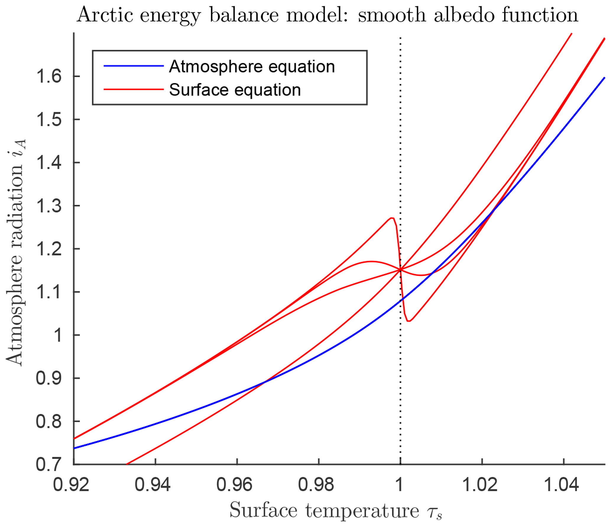
Figure A1Graphs of the nondimensionalized EBM Eqs. (6)–(6). The red curves represent the surface EBM Eq. (6). The smooth red curves represent α(TS) as in Eq. (A3), with , on successively flatter red curves. The blue curve represents the atmosphere Eq. (6). There are up to three intersections of the blue curve Eq. (6) with a given red curve Eq. (6) in this figure. Other parameters in the EBM are αC=0.7, αW=0.08, δ=0.67, μ=400, , and Z=9 km.
Figure A1 shows the nondimensional energy balance Eq. (6) (in blue) and Eq. (6) (in red) for a range of values of the parameter in Eq. (A3). The blue (atmosphere) curve may have up to three intersections with a red (surface) curve, implying the existence of multiple equilibrium states.
A3 Average global surface temperature
Both Wild et al. (2013) and Trenberth et al. (2009) indicate that the globally averaged amount of infrared radiation being emitted by the surface of the Earth is 398 W m−2. Since the EBM assumes the Earth is a black-body radiator, the Stefan–Boltzmann law dictates that the corresponding temperature is
This temperature is equivalent to 16.3 ∘C, which is a little higher than the accepted average surface temperature of about 14 ∘C. This is not surprising since the former is obtained by essentially averaging T4 while the latter is obtained from averaging actual temperatures. We use the above value for in the calibrations described below, since it is consistent with the EBM.
A4 Heat convection/conduction and evapotranspiration
Evapotranspiration (ET) is the transport of water from the surface to the atmosphere in the form of water vapour. It combines the effects of evaporation from the surface and transpiration by plants. Globally, the largest contributor is evaporation from the surface of the oceans and the main determining factor there is the ocean surface temperature. The ET process also transports heat from the surface to the atmosphere, in the form of latent heat. Recently Wang et al. (2010) have shown that global ET has been increasing over the past several decades.
The forcing term FC in the EBM represents transport of heat away from the surface to the atmosphere by conduction plus convection plus change of state of water. The most important of these is the upward transport of latent heat. Surface water evaporates, taking heat from the surface. As warm moist air rises and cools, the water vapour condenses, releasing its latent heat into the surrounding atmosphere. According to both Wild et al. (2013) and Trenberth et al. (2009), the magnitude of this forcing is . However, this is a globally averaged value and, due to strong dependence on temperature, is not likely valid at temperatures other than the globally averaged surface temperature . In the past several decades, ET has increased by 0.6 W m−2 per decade (Wang et al., 2010). Extrapolating back 100 years, this would be 6 W m−2. In the past century the average global surface temperature has risen about 1 ∘C. Thus it is reasonable to assume the dependence of FC on the surface temperature TS should have a slope near of about 6. If the dependence of FC on TS was simply linear, then, given that , this slope would predict that FC was negative for ∘C. Since negative values for FC are unreasonable, and since there likely is still some heat transport even near freezing, instead of a linear function, we have modelled the dependence of FC on temperature as a hyperbolic function that is nearly zero for temperatures below freezing, and increases roughly linearly for temperatures above freezing. Specifically, we use the function
or equivalently,
where A1 and A2 are constants. In terms of the nondimensional variables and parameters Eq. (6), this equation becomes
The constants A1 and A2 are chosen so that the forcing at the global average surface temperature is 104, and so that the forcing at the freezing point is 20 % of this value, that is, . Thus
or in terms of the nondimensional parameters,
Figure A2 shows a plot of Eq. (A5) for these parameter values. With these choices of the constants, the slope at is 5.9, agreeing well with the above argument that it should be about 6.
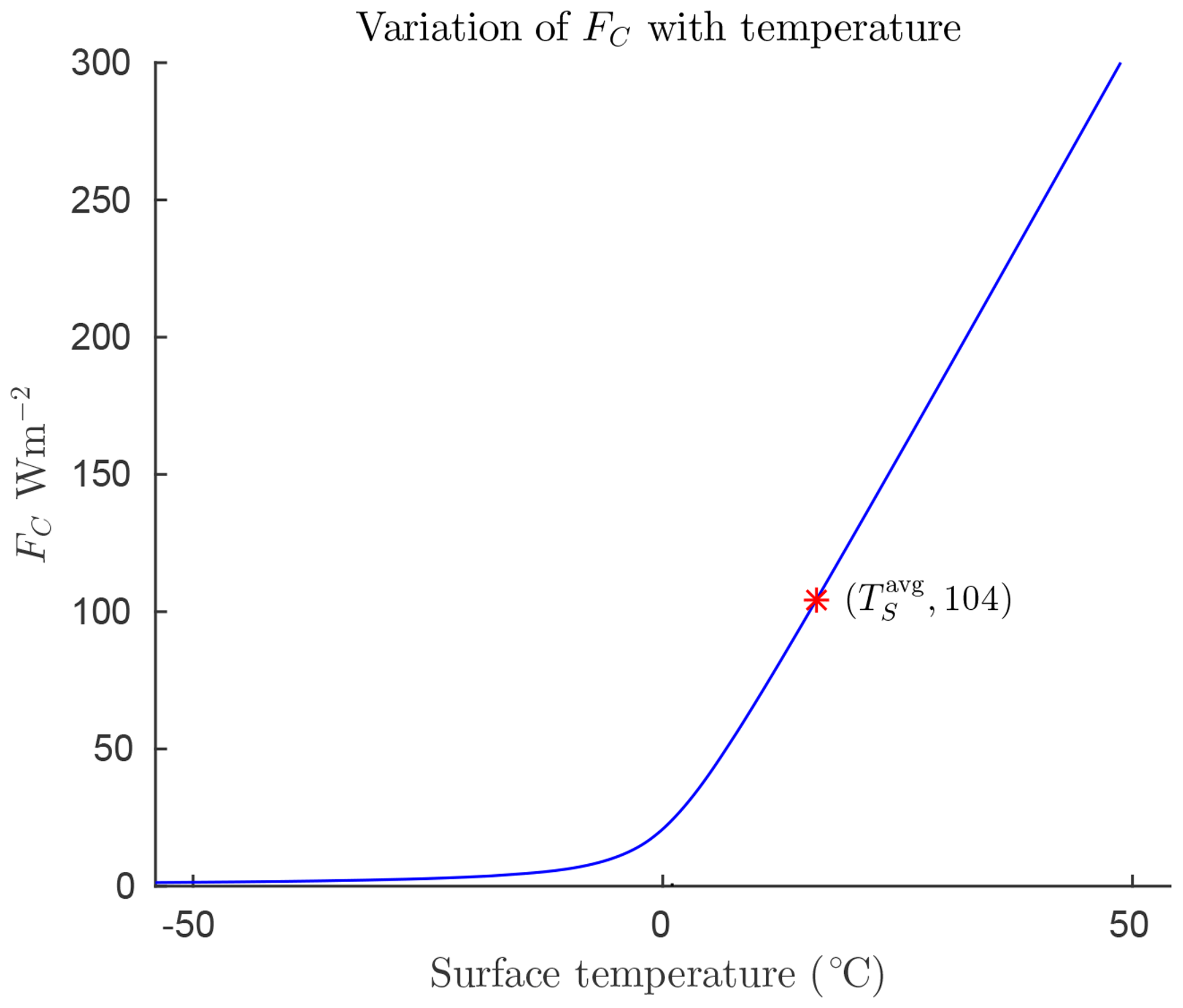
Figure A2Variation of evapotranspiration/convection with surface temperature. The hyperbolic function is tangent to the horizontal as the temperature decreases, and grows almost linearly with a slope of about 6 as temperature increases.
A5 Atmospheric absorption of infrared radiation
Two of the empirical parameters in the EBM are kW and kC, defined in Sect. 2.2 as the grey gas absorption coefficients for water vapour and carbon dioxide, respectively. More precisely, the absorption coefficient k of a gas is its proportionality coefficient in the Beer–Lambert law, as defined in Eq. (6) of Sect. 2.2. In the grey gas approximation, it is assumed that the absorption coefficient k is constant for all frequencies of incident radiation, and depends only on the total intensity of that radiation. In reality though, k is not an absolute physical constant because gases absorb radiation at discrete spectral lines. The total amount of energy absorbed depends on the distribution of energy in the radiation at each of these spectral wavelengths. Values of kW and kC for the particular spectrum of incident radiation experienced by the atmosphere may be obtained empirically from modern era satellite and land-based measurements. We assume that kW and kC for the atmosphere do not change with time, even over the geological timescales considered here.
Atmospheric absorption, η, of infrared radiation emitted by the Earth is, in this EBM, attributed to the two primary greenhouse gases: water vapour and carbon dioxide, and to the liquid and solid water making up clouds. According to Trenberth et al. (2009), at present as a global average, the Earth emits 398 W m−2 of which 40.1 W m−2 passes through the atmosphere to space. Thus approximately 90 % of the radiation is absorbed in the atmosphere, that is η=0.9. The present-day absorption factor η can be attributed as follows (Schmidt et al., 2010): water vapour 50 %, clouds 25 % and CO2 (plus other gases) 25 %. Furthermore, they determined that these ratios remain unchanged, even after a doubling of CO2. Therefore, setting and ηW=2x in Eq. (10) we get
This cubic has one real root, ,
In this model, since we have no data on cloud cover for paleoclimates, we make the assumption that absorption due to clouds is a constant globally and temporally, and set
We also tried varying ηCl with temperature using a hyperbolic function like that used for FC in Eq. (A5); however, we found no qualitative change in the results and therefore, for simplicity, have left ηCl as a constant. To calibrate the absorption coefficient kC for the greenhouse gas carbon dioxide, we set in Eq. (14) yielding
Using the present-day value of μ=400 ppm, the value of from Eq. (A7), the standard atmospheric pressure value of , and the acceleration due to gravity we get
With this value for kC, the coefficient GC, defined in Eq. (13) has the value
To calibrate kW we proceed as follows. The latent heat of vaporization of water is and the ideal-gas constant specific to water vapour is . Thus from Eq. (24) we have
Dai (2006) indicates that an average value for relative humidity, δ, from 1976 to 2004 for the region of the Earth between 60∘ S and 75∘ N is 0.74. Over the same latitudes, Dai reports that averages over water and over land are 0.79 and 0.65, respectively, except that over deserts the humidity drops to 30 %–50 %. The polar regions are typically drier; however, there is a significant amount of water north of 75∘ N and south of 60∘ S, hence we have chosen δavg=0.74 as the average global relative humidity for purposes of calibrating kW. In Eq. (25) we set with given by Eq. (A7), τS to the present normalized global average temperature , δ to the present average global relative humidity δavg, Z to an average global tropopause height of Zavg=14000 m, and the normalized lapse rate to . Using these values and inverting Eq. (25) to isolate kW we get
With this value for kW, the second greenhouse gas parameter for water vapour is
A6 Atmospheric emission of radiation
In previous slab models, including Dortmans et al. (2018) and Payne et al. (2015), it was assumed that the upward and downward radiation intensities from the atmosphere are equal; that is, in Eq. (1). This would be the case for an actual uniform slab; however, the real atmosphere is not uniform in temperature nor density, and in fact both the temperature and density of the atmosphere are much higher in value near the surface than near the tropopause. The net effect of this nonuniformity is that, of the total radiation intensity IA emitted by the atmosphere, almost two-thirds goes back to the surface and only a little more than one-third escapes to space, according to satellite and surface data (Trenberth et al., 2009; Wild et al., 2013). From Trenberth et al. (2009), the atmosphere and clouds emit upward to space and emit 340.3 W m−2 downward to the Earth. Therefore, in order to have the model in this paper represent the atmosphere more realistically, we set
instead of 0.50.
Equilibrium climate sensitivity (ECS) is a useful measure of the sensitivity of a given climate model to an increase in CO2 concentration μ. It is usually defined as the change ΔT in the global mean temperature , resulting from a doubling of μ, starting from the accepted pre-industrial value μ=270 ppm (IPCC, 2013; Forster, 2016; Knutti et al., 2017; Proistosescu and Huybers, 2017). The ECS provides a first-order estimate of the amount of present-day global warming predicted by a given model as μ increases. Because ECS is a single number, it facilitates comparisons between models. It has been used extensively in the assessment reports of the IPCC (IPCC, 2013), where ΔT values in the range 1.5 to 4.5 ∘C have been documented. Some have cited this wide range of ECS values as a sign of weakness of the IPCC methodology. Recently these results have been reconciled (Proistosescu and Huybers, 2017). They showed that a linear statistical analysis of historical data gives low estimates in the 1.5 to 3 ∘C range, while nonlinear models give higher estimates.
In terms of our EBM, to apply it to a global average we make the following settings. The global mean insolation at the top of the atmosphere is (Wild et al., 2013; Trenberth et al., 2009). They indicate that 161 W m−2 of sunlight is absorbed by the Earth while 24 W m−2 is reflected back on average. Thus we take
For the tropopause height Z we take an average value of Zavg=14 km. For the global model, the ocean and atmospheric transport terms, FO and FA, will be zero.
The ECS value we calculate will be the difference between the warm equilibrium temperatures when μ=270 and μ=540. For these calculations we took the relative humidity to be , in accord with the value obtained in Dai (2006). The graphs of the surface and atmosphere equilibrium equations are shown in Fig. B1. The equilibrium solutions of this global mean version of the EBM yield TS(270)=14.3, TS(540)=17.6 and ΔT=3.3 ∘C. This is in excellent agreement with accepted values (IPCC, 2013).
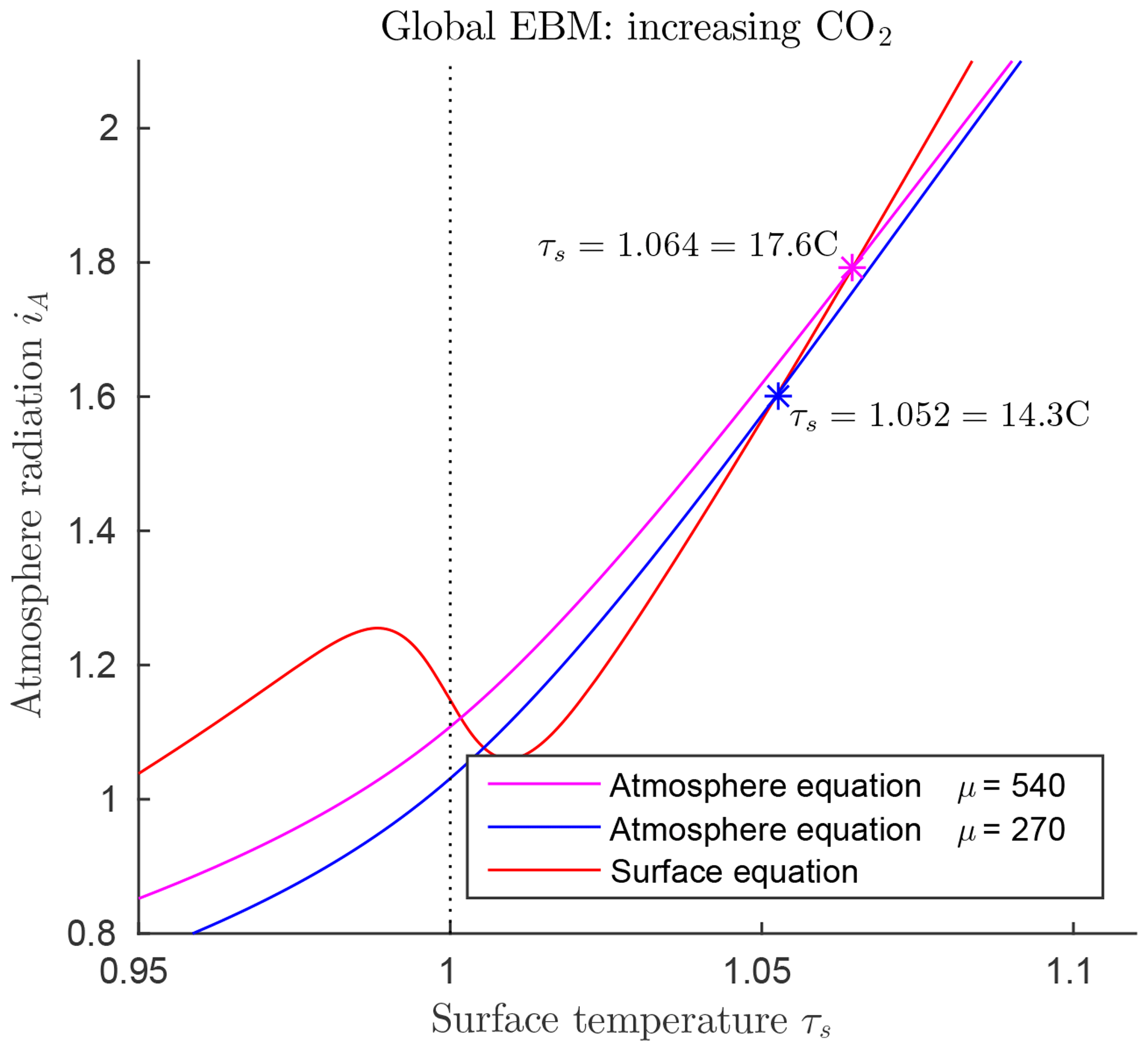
Figure B1Equilibrium climate sensitivity (ECS) for millennial data. The equilibrium points marked with stars show the change in TS for a doubling of μ from 270 to 540 ppm; TS(270)=14.3, TS(540)=17.6 and ΔT=3.3 ∘C.
WFL contributed the original hypothesis on which the investigation is based, guided the work and wrote much of the original paper. BD carried out the computations required for this research and wrote an MSc thesis on his work, which was the starting point for this paper. ARW co-supervised BD's work, significantly extended his calculations, contributed many insights and guidance for this paper, and wrote much of the major revision of this paper.
The authors declare that they have no conflict of interest.
The authors acknowledge financial support of this work by the Natural Sciences and Engineering Research Council of Canada, and thank two anonymous referees for many valuable suggestions that greatly improved the quality of the paper. The authors thank Kolja Kypke for his contributions to the final revisions of the manuscript. William F. Langford gratefully acknowledges very helpful discussions with James F. Basinger and David R. Greenwood in the early stages of this work.
This paper was edited by Qiuzhen Yin and reviewed by two anonymous referees.
Alley, R. B., Marotzke, J., Nordhaus, W. D., Overpeck, J. T., Peteet, D. M., Pielke Jr., A., Pierrehumbert, R. T., Rhines, P. B., Stocker, T. F., Talley, L. D., and Wallace, J. M.: Abrupt climate change, Science, 299, 2005–2010, 2003. a
Arnold, L., Namachchivaya, N. S., and Schenk, K.: Toward an understanding of stochastic bifurcation: Case study, Internat. J. Bifur. Chaos, 6, 1947–1979, 1996. a
Baatsen, M., von der Heydt, A. S., Huber, M., Kliphuis, M. A., Bijl, P. K., Sluijs, A., and Dijkstra, H. A.: Equilibrium state and sensitivity of the simulated middle-to-late Eocene climate, Clim. Past Discuss., https://doi.org/10.5194/cp-2018-43, in review, 2018. a
Ballantyne, A. P., Greenwood, D. R., Sinninghe Damsté, J. S., Csank, A. Z., Eberle, J. J., and Rybczynski, N.: Significantly Warmer Arctic Surface Temperatures during the Pliocene Indicated by Multiple Independent Proxies, Geology, 38, 603–606, 2010. a, b, c
Barron, E. J.: A warm, equable Cretaceous: the nature of the problem, Earth-Sci. Rev., 19, 305–338, 1983. a, b, c, d, e, f
Barron, E. J., Thompson, S. L., and Schneider, S. H.: An Ice-Free Cretaceous? Results from Climate Model Simulations, Science, 212, 501–508, 1981. a, b, c, d, e, f, g, h, i, j, k
Barron, E. J., Fawcett, P. J., Peterson, W. H., Pollard, D., and Thompson, S. L.: A “simulation” of mid-Cretaceous climate, Paleoceanography, 10, 953–962, 1995. a, b, c
Bartoli, G., Sarnthein, M., Weinelt, M., Erlenkeuser, H., Garbe-Schönberg, D., and Lea, D. W.: Final closure of Panama and the onset of northern hemisphere glaciation, Earth Planet. Sc. Lett., 237, 33–44, 2005. a
Bartoli, G., Hönisch, B., and Zeebe, R. E.: Atmospheric CO2 decline during the Pliocene intensification of Northern Hemisphere glaciations, Paleoceanography, 26, PA4213, https://doi.org/10.1029/2010PA002055, 2011. a
Basinger, J. F., Greenwood, D. R., and Sweda, T.: Early Tertiary vegetation of Arctic Canada and its relevance to Paleoclimatic interpretation, in: Cenozoic Plants and Climate of the Arctic, NATO ASI Series, Vol. 127, edited by: Boulter, M. C. and Fisher, H. C., 175–198, Springer-Verlag, 1994. a
Bice, K. L., Birgel, D., Meyers, P. A., Dahl, K. A., Hinrichs, K.-U., and Norris, R. D.: A multiple proxy and model study of Cretaceous upper ocean temperatures and atmospheric CO2 concentrations, Paleoceanography, 21, PA2002, https://doi.org/10.1029/2005PA001203, 2006. a, b
Bowman, V. C., Francis, J. E., Askin, R. A., Riding, J. B., and Swindles, G. T.: Latest Cretaceous – earliest Paleogene vegetation and climate change at the high southern latitudes: Palynological evidence from Seymour Island, Antarctic Peninsula, Palaeogeogr. Palaeocl., 408, 26–47, 2014. a
Brierley, C., Burls, N., Ravelo, C., and Fedorov, A.: Pliocene warmth and gradients, Nat. Geosci., 8, 419–420, 2015. a
Briggs, J. C.: Biogeography and Plate Tectonics, Elsevier, Amsterdam, 1987. a, b
Budyko, M. I.: The effect of solar radiation variations on the climate of the Earth, Tellus, 21, 611–619, 1968. a, b
Calov, R. and Ganopolski, A.: Multistability and hysteresis in the climate-cryosphere system under orbital forcing, Geophys. Res. Lett., 32, L21717, https://doi.org/10.1029/2005GL024518, 2005. a
Chandan, D. and Peltier, W. R.: Regional and global climate for the mid-Pliocene using the University of Toronto version of CCSM4 and PlioMIP2 boundary conditions, Clim. Past, 13, 919–942, https://doi.org/10.5194/cp-13-919-2017, 2017. a, b
Chandan, D. and Peltier, W. R.: On the mechanisms of warming the mid-Pliocene and the inference of a hierarchy of climate sensitivities with relevance to the understanding of climate futures, Clim. Past, 14, 825–856, https://doi.org/10.5194/cp-14-825-2018, 2018. a, b
Claussen, M., Kubatzki, C., Brovkin, V., and Ganopolski, A.: Simulation of an abrupt change in Saharan vegetation in the Mid-Holocene, Geophys. Res. Lett., 26, 2037–2040, 1999. a
Craggs, H. J., Valdes, P. J., and Widdowson, M.: Climate model predictions for the latest Cretaceous: An evaluation using climatically sensitive sediments as proxy indicators, Palaeogeogr. Palaeocl., 315, 12–23, 2012. a
Cronin, T. M.: Paleoclimates: Understanding Climate Change Past and Present, Columbia University Press, New York, 2010. a, b, c, d, e, f, g, h, i, j, k
Crowley, T. J.: Carbon dioxide and Phanerozoic climate, in: Warm Climates in Earth History, edited by: Hubert, B. T., MacLead, K. G., and Wing, S. L., 425–444, Cambridge Univ. Press, Cambridge, UK, 2000. a
Csank, A. Z., Patterson, W. P., Eglington, B. M., Rybczynski, N., and Basinger, J. F.: Climate variability in the Early Pliocene Arctic: Annually resolved evidence from stable isotope values of sub-fossil wood, Ellesmere Island, Canada, Palaeogeogr. Palaeocl., 398, 339–349, 2011. a
Dai, A.: Recent Climatology, Variability, and Trends in Global Surface Humidity, J. Climate, 19, 3589–3606, https://doi.org/10.1175/JCLI3816.1, 2006. a, b
DeConto, R. M., Pollard, D., Wilson, P. A., Pälike, H., Lear, C. H., and Pagani, M.: Thesholds for Cenozoic Bipolar Glaciation, Nature, 455, 652–657, 2008. a, b, c
De Schepper, S., Groeneveld, J., Naafs, B. D. A., Van Renterghem, C., Hennissen, J., Head, M. J., Louwye, S., and Fabian, K.: Northern hemisphere glaciation during the globally warm early late Pliocene, PLoS ONE, 8, e81508, https://doi.org/10.1371/journal.pone.0081508 , 2013. a, b
De Schepper, S., Schreck, M., Beck, K. M., Matthiessen, J., Fahl, K., and Mangerud, G.: Early Pliocene onset of modern Nordic Seas circulation related to ocean gateway changes, Nat. Commun., 6, 1–8, https://doi.org/10.1038/ncomms9659, 2015. a, b
Donnnadieu, Y., Pierrehumbert, R., Jacob, R., and Fluteau, F.: Modelling the primary control of paleogeography on Cretaceous climate, Earth Planet. Sc. Lett., 248, 426–437, 2006. a, b
Dortmans, B.: A Conceptual Model of Climate Change Incorporating the Roles of Carbon Dioxide and Water Vapour as Greenhouse Gases, Master's thesis, Department of Mathematics and Statistics, University of Guelph, 2017. a, b, c
Dortmans, B., Langford, W. F., and Willms, A. R.: A Conceptual Model for the Pliocene Paradox, in: Recent Advances in Mathematical and Statistical Methods for Scientific and Engineering Applications, edited by: Kilgour, D. M., Kunze, H., Makarov, R., Melnik, R., and Wang, S., 339–349, Springer Nature, AMMCS 2017, Waterloo, Canada, https://doi.org/10.1007/978-3-319-99719-3_31, 2018. a, b, c, d
Dowsett, H., Dolan, A., Rowley, D., Moucha, R., Forte, A. M., Mitrovica, J. X., Pound, M., Salzmann, U., Robinson, M., Chandler, M., Foley, K., and Haywood, A.: The PRISM4 (mid-Piacenzian) paleoenvironmental reconstruction, Clim. Past, 12, 1519–1538, https://doi.org/10.5194/cp-12-1519-2016, 2016. a
Dowsett, H. J., Haywood, A. M., Valdes, P. J., Robinson, M. M., Lunt, D. J., Hill, D. J., Stoll, D. K., and Foleya, K. M.: Sea surface temperatures of the mid-Piacenzian Warm Period: A comparison of PRISM3 and HadCM3, Palaeogeogr. Palaeocl., 309, 83–91, 2011. a, b
Dowsett, H. J., Robinson, M. M., Stoll, D. K., Foley, K. M., Johnson, A. L., Williams, M., and Riesselman, C. R.: The PRISM (Pliocene palaeoclimate) reconstruction: time for a paradigm shift, Philos. T. Roy. Soc. A, 371, 2012524, https://doi.org/10.1098/rsta.2012.0524, 2013. a
Fedorov, A. V., Dekens, P. S., McCarthy, M., Ravelo, A. C., deMenocal, P. B., Barreiro, M., Pacanowski, R. C., and Philander, S. G.: The Pliocene Paradox (Mechanisms for a Permanent El Niño), Science, 312, 1485–1489, https://doi.org/10.1126/science.1122666, 2006. a, b, c, d
Fedorov, A. V., Brierley, C. M., and Emanuel, K.: Tropical cyclones and permanent El Niño in the early Pliocene epoch, Nature, 463, 1066–1070, 2010. a, b, c, d
Ferreira, D., Marshall, J., and Rose, B.: Climate Determinism Revisted: Multiple Equilibria in a Complex Climate Model, J. Climate, 24, 992–1012, 2010. a
Fletcher, B. J., Brentnall, S. J., Anderson, C. W., Bemer, R. A., and Beerling, D. J.: Atmospheric Carbon Dioxide Linked with Mesozoic and early Cenozoic Climage Change, Nat. Geosi., 1, 43–48, 2008. a, b, c
Fletcher, T., Warden, L., Sinninghe Damsté, J. S., Brown, K. J., Rybczynski, N., Gosse, J., and Ballantyne, A. P.: The role of elevated atmospheric CO2 and increased fire in Arctic amplification of temperature during the Early to mid-Pliocene, Clim. Past Discuss., https://doi.org/10.5194/cp-2018-60, in review, 2018. a, b
Forster, P. M.: Inference of Climate Sensitivity from Analysis of Earth's Energy Budget, Annu. Rev. Earth Pl. Sc., 44, 85–106, 2016. a
Fretwell, P., Pritchard, H. D., Vaughan, D. G., Bamber, J. L., Barrand, N. E., Bell, R., Bianchi, C., Bingham, R. G., Blankenship, D. D., Casassa, G., Catania, G., Callens, D., Conway, H., Cook, A. J., Corr, H. F. J., Damaske, D., Damm, V., Ferraccioli, F., Forsberg, R., Fujita, S., Gim, Y., Gogineni, P., Griggs, J. A., Hindmarsh, R. C. A., Holmlund, P., Holt, J. W., Jacobel, R. W., Jenkins, A., Jokat, W., Jordan, T., King, E. C., Kohler, J., Krabill, W., Riger-Kusk, M., Langley, K. A., Leitchenkov, G., Leuschen, C., Luyendyk, B. P., Matsuoka, K., Mouginot, J., Nitsche, F. O., Nogi, Y., Nost, O. A., Popov, S. V., Rignot, E., Rippin, D. M., Rivera, A., Roberts, J., Ross, N., Siegert, M. J., Smith, A. M., Steinhage, D., Studinger, M., Sun, B., Tinto, B. K., Welch, B. C., Wilson, D., Young, D. A., Xiangbin, C., and Zirizzotti, A.: Bedmap2 : improved ice bed, surface and thickness datasets for Antarctica, The Cryosphere, 7, 375–393, https://doi.org/10.5194/tc-7-375-2013, 2013. a
Ganopolski, A. and Rahmstorf, S.: Rapid changes of glacial climate simulated in a coupled climate model, Nature, 409, 153–158, 2001. a, b
Goldner, A., Herold, N., and Huber, M.: Antarctic Glaciation Caused Ocean Circulation Chages at the Eocene-Oligocene Transition, Nature, 511, 574–577, 2014. a, b, c, d
Greenwood, D. R., Basinger, J. F., and Smith, R. Y.: How wet was the Arctic Eocene rain forest? Estimates of precipitation from Paleogene Arctic macrofloras, Geology, 38, 15–18, 2010. a, b
Haug, G. H., Tiedemann, R., and Keigwin, L. D.: How the Isthmus of Panama put ice in the Arctic, Oceanus, 42, 1–4, 2004. a, b
Haywood, A. M., Dowsett, H. J., Valdes, P. J., Lunt, D. J., Francis, J. E., and Sellwood, B. W.: Introduction. Pliocene climate, processes and problems, Philos. T. Roy. Soc. A, 367, 3–17, 2009. a, b, c, d
Haywood, A. M., Dowsett, H. J., Robinson, M. M., Stoll, D. K., Dolan, A. M., Lunt, D. J., Otto-Bliesner, B., and Chandler, M. A.: Pliocene Model Intercomparison Project (PlioMIP): experimental design and boundary conditions (Experiment 2), Geosci. Model Dev., 4, 571–577, https://doi.org/10.5194/gmd-4-571-2011, 2011. a
Haywood, A. M., Dowsett, H. J., Dolan, A. M., Rowley, D., Abe-Ouchi, A., Otto-Bliesner, B., Chandler, M. A., Hunter, S. J., Lunt, D. J., Pound, M., and Salzmann, U.: The Pliocene Model Intercomparison Project (PlioMIP) Phase 2: scientific objectives and experimental design, Clim. Past, 12, 663–675, https://doi.org/10.5194/cp-12-663-2016, 2016. a
Huber, M. and Caballero, R.: The early Eocene equable climate problem revisited, Clim. Past, 7, 603–633, https://doi.org/10.5194/cp-7-603-2011, 2011. a, b, c, d, e
Hubert, B. T., MacLead, K. G., and Wing, S. L.: Warm Climates in Earth History, Cambridge Univ. Press, Cambridge, UK, 2000. a
Hutchinson, D. K., de Boer, A. M., Coxall, H. K., Caballero, R., Nilsson, J., and Baatsen, M.: Climate sensitivity and meridional overturning circulation in the late Eocene using GFDL CM2.1, Clim. Past, 14, 789–810, https://doi.org/10.5194/cp-14-789-2018, 2018. a, b
Intergovernmental Panel on Climate Change: Climate Change 2013: The Physical Science Basis, in: Contribution of Working Group I to the Fifth Assessment Report of the Intergovernmental Panel on Climate Change, edited by: Stocker, T. F., Qin, D., Plattner, G. K., Tignor, M., Allen, S. K., Boschung, J., Nauels, A., Xia, Y., Bex, V., and Midgley, P. M., Cambridge Univ. Press, Cambridge, UK and New York, NY, USA, available at: http://www.ipcc.ch/ (last access: 11 March 2019), 2013. a, b, c, d, e, f, g
International Civil Aviation Organization: Manual of the ICAO Standard Atmosphere, Extended to 80 kilometres, 1000 Sherbrooke Street West Suite 400, Montreal, Quebec, Canada H3A 2R2, third edn., 1993. a, b, c
Jahren, A. H. and Sternberg, L. S. L.: Humidity estimate for the middle Eocene Arctic rain forest, Geology, 31, 463–466, 2003. a, b, c, d
Kaper, H. and Engler, H.: Mathematics and Climate, Society for Industrial and Applied Mathematics, Philadelphia, USA, 2013. a, b, c
Katz, M. E., Miller, K. G., Wright, J. D., Wade, B. S., Browning, J. V., Cramer, B. S., and Rosenthal, Y.: Stepwise transition from the Eocene greenhouse to the Oligocene icehouse, Nat. Geosci., 1, 329–334, 2008. a
Kishore, P., Namboothiri, S. P., Igarashi, K., Jiang, J. H., Ao, C. O., and Romans, L. J.: Climatological Characteristics of the Tropopause Parameters Derived from GPS/CHAMP and GPS/SAC-C Measurements, J. Geophys. Res., 111, D20110, https://doi.org/10.1029/2005JD006827, 2006. a, b
Knies, J., Cabedo-Sanz, P., Belt, S. T., Baranwal, S., Fietz, S., and Rosell-Melé, A.: The emergence of modern sea ice cover in the Arctic Ocean, Nat. Commun., 5, 5608, https://doi.org/10.1038/ncomms6608, 2014. a, b
Knutti, R., Rugenstein, M. A., and Hegerl, G. C.: Beyond equilibrium climate sensitivity, Nat. Geosci., 10, 727–736, 2017. a
Kuznetsov, Y. A.: Elements of Applied Bifurcation Theory, Springer, New York, third edn., 2004. a, b
Ladant, J. B. and Donnadieu, Y.: Palaeogeographic regulation of glacial events during the Cretaceous supergreenhouse, Nat. Commun., 7, 12771, https://doi.org/10.1038/ncomms12771, 2016. a, b
Ladant, J. B., Donnadieu, Y., Lefebvre, V., and Dumas, C.: The respective role of atmospheric carbon dioxide and orbital parameters on ice sheet evolution at the Eocene-Oligocene transition, Paleoceanography, 29, 810–823, 2014. a, b, c
Langford, W. F. and Lewis, G. M.: Poleward expansion of Hadley cells, Can. Appl. Math. Quart., 17, 105–119, 2009. a
Lawrence, K. T., Herbert, T. D., Brown, C. M., Raymo, M. E., and Haywood, A. M.: High-amplitude variations in North Atlantic sea surface temperature during the early Pliocene warm period, Paleoceanography, 24, PA2218, https://doi.org/10.1029/2008PA001669, 2009. a
Lear, C. H., Bailey, T. R., Pearson, P. N., Coxall, H. K., and Rosenthal, Y.: Cooling and ice growth across the Eocene-Oligocene transition, Geology, 36, 251–254, 2008. a, b
Lenton, T. M., Livina, V. N., Dakos, V., and Scheffer, M.: Climate bifurcation during the last deglaciation?, Clim. Past, 8, 1127–1139, https://doi.org/10.5194/cp-8-1127-2012, 2012. a
Lewis, G. M. and Langford, W. F.: Hysteresis in a rotating differentially heated spherical shell of Boussinesq fluid, SIAM J. Appl. Dyn. Syst., 7, 1421–1444, 2008. a
Lindsay, R. W. and Zhang, J.: The thinning of Arctic sea ice, 1988–2003: have we passed a tipping point?, J. Climate, 18, 4979–4896, 2005. a
Liu, Z., Otto-Bliesner, B. L., He, F., Brady, E. C., Tomas, R., Clark, P. U., Carlson, A. E., Lynch-Stieglitz, J., Curry, W., Brook, E., Erickson, D., Jacob, R., Kutzbach, J., and Cheng J.: Transient simulation of last deglaciation with a new mechanism for Bolling-Allerod warming, Science, 325, 310–314, 2009. a
Lunt, D. J., Foster, G. L., Haywood, A. M., and Stone, E. J.: Late Pliocene Greenland glaciation controlled by a decline in atmospheric CO2 levels, Nature, 454, 1102–1105, 2008. a, b
Lunt, D. J., Farnsworth, A., Loptson, C., Foster, G. L., Markwick, P., O'Brien, C. L., Pancost, R. D., Robinson, S. A., and Wrobel, N.: Palaeogeographic controls on climate and proxy interpretation, Clim. Past, 12, 1181–1198, https://doi.org/10.5194/cp-12-1181-2016, 2016. a, b
Lunt, D. J., Huber, M., Anagnostou, E., Baatsen, M. L. J., Caballero, R., DeConto, R., Dijkstra, H. A., Donnadieu, Y., Evans, D., Feng, R., Foster, G. L., Gasson, E., von der Heydt, A. S., Hollis, C. J., Inglis, G. N., Jones, S. M., Kiehl, J., Kirtland Turner, S., Korty, R. L., Kozdon, R., Krishnan, S., Ladant, J.-B., Langebroek, P., Lear, C. H., LeGrande, A. N., Littler, K., Markwick, P., Otto-Bliesner, B., Pearson, P., Poulsen, C. J., Salzmann, U., Shields, C., Snell, K., Stärz, M., Super, J., Tabor, C., Tierney, J. E., Tourte, G. J. L., Tripati, A., Upchurch, G. R., Wade, B. S., Wing, S. L., Winguth, A. M. E., Wright, N. M., Zachos, J. C., and Zeebe, R. E.: The DeepMIP contribution to PMIP4: experimental design for model simulations of the EECO, PETM, and pre-PETM (version 1.0), Geosci. Model Dev., 10, 889–901, https://doi.org/10.5194/gmd-10-889-2017, 2017. a
McGehee, R. and Lehman, C.: A paleoclimate model of ice-albedo feedback forced by variations in Earth's orbit, SIAM J. Appl. Dynam. Syst., 11, 684–707, 2012. a, b, c, d
Miller, K. G., Browning, J. V., Aubry, M.-P., Wade, B. S., Katz, M. E., Kulpecz, A. A., and Wright, J. D.: Eocene-Oligocene global climate and sea-level changes: St. Stephens Quarry, Alabama, GSA Bulletin, 120, 34–53, 2008. a, b, c
Namachchivaya, N. S.: Stochastic Bifurcations, J. Appl. Math. Comput., 38, 101–159, 1990. a
North, G. R., Cahalan, R. F., and Coakley, J. A.: Energy balance climate models, Rev. Geophys. Space Ge., 19, 91–121, 1981. a, b
O'Brien, C. L., Foster, G. L., Martinez-Botí, M. A., Abell, R., Rae, J. W., and Pancost, R. D.: High sea surface temperatures in tropical warm pools during the Pliocene, Nat. Geosci., 7, 606–611, 2014. a
O'Brien, C. L., Robinson, S. A., Pancost, R. D., Damsté, J. S. S., Schouten, S., Lunt, D. J., Alsenz, H., Bornemann, A., Bottini, C., Brassell, S. C., Farnsworth, A., Forster, A., Huber, B. T., Inglis, G. N., Jenkyns, H. C., Linnert, C., Littler, K., Markwick, P., McAnena, A., Mutterlose, J., Naafs, B. D. A., Püttmann, W., Sluijs, A., van Helmond, N. A. G. M., Vellekoop, J., Wagner, T., and Wrobel, N. E.: Cretaceous sea-surface temperature evolution: Constraints from TEX86 and planktonic foraminiferal oxygen isotopes, Earth Sci. Rev., 172, 224–247, 2017. a, b
Pagani, M., Arthur, M. A., and Freeman, K. H.: Miocene evolution of atmospheric carbon dioxide, Paleoceanography, 14, 273–292, 1999. a
Pagani, M., Zachos, J. C., Freeman, K. H., Tipple, B., and Bohaty, S.: Marked decline in atmospheric carbon dioxide concentrations during the Paleogene, Science, 309, 600–603, 2005. a, b, c, d, e, f, g
Pagani, M., Caldeira, K., Archer, D., and Zachos, K. C.: An ancient carbon mystery, Science, 34, 1556–1557, 2006. a, b
Pagani, M., Huber, M., Liu, Z., Bohaty, S. M., Henderiks, J., Sijp, W., Krishnan, S., and DeConto, R. N.: The role of carbon dioxide during the onset of Antarctic glaciation, Science, 334, 1261–1264, 2011. a, b, c, d
Paillard, D.: The timing of Pleistocene glaciations from a simple multiple-state climate model, Nature, 391, 378–381, 1998. a
Paillard, D.: Glacial hiccups, Nature, 409, 147–148, 2001. a
Paillard, D.: Glacial cycles: toward a new paradigm, Rev. Geophys., 39, 325–346, 2001. a
Payne, A. E., Jansen, M. F., and Cronin, T. W.: Conceptual model analysis of the influence of temperature feedbacks on polar amplification, Geophys. Res. Lett., 42, 9561–9570, 2015. a, b, c, d
Pierrehumbert, R. T.: Principles of Planetary Climate, Cambridge University Press, Cambridge, UK, 2010. a, b, c
Proistosescu, C. and Huybers, P. J.: Slow climate mode reconciles historical and model-based estimates of climate sensitivity, Sci. Adv., 3, e1602821, https://doi.org/10.1126/sciadv.1602821, 2017. a, b
Rahmstorf, S.: Bifurcations of the Atlantic thermohaline circulation in response to changes in the hydrological cycle, Nature, 378, 145–149, 1995. a
Rial, J. A., Pielke Sr., R. A., Beniston, M., Claussen, M., Canadell, J., Cox, P., Held, H., De Noblet-Ducoudrè, N., Prinn, R., Reynolds, J. F., and Salas, J. D.: Nonlinearities, Feedbacks and critical thresholds within the Earth's climate system, Climate Change, 65, 11–38, 2004. a
Robinson, A., Calov. R., and Ganopolsky, A.: Multistability and critical thresholds of the Greenland ice sheet, Nat. Clim. Change, 2, 429–432, 2012. a
Ruddiman, W. F.: Earth's Climate Past and Future, W. H. Freeman and Company, third edn., 2014. a, b
Sagan, C. and Mullen, G.: Earth and Mars: Evolution of atmospheres and surface temperatures, Science, New Series, 177, 52–56, 1972. a, b
Salzmann, U., Haywood, A. M., and Lunt, D. J.: The past is a guide to the future? Comparing Middle Pliocene vegetation with predicted biome distributions for the twenty-first century, Phil. T. Roy. Soc. A, 367, 189–204, 2009. a, b
Scher, H. D., Bohaty, S. M., Zachos, J. C., and Delany, M. L.: Two-stepping into the icehouse: East Antarctic weathering during progressive ice-sheet expansion at the Eocene–Oligocene transition, Geology, 39, 383–386, 2011. a, b, c
Scher, H. D., Whittaker, J. M., Williams, S. E., Latimer, J. C., Kordesch, W. E. C., and Delaney, M. L.: Onset of Antartic Circumpolar Current 30 Million Years Ago as Tasmanian Gateway Aligned with Westerlies, Nature, 523, 580–583, 2015. a, b, c, d, e, f
Schmidt, G. A., Ruedy, R. A., Miller, R. L., and Lacis, A. A.: Attribution of the present-day total greenhouse effect, J. Geophys. Res., 115, D20106, https://doi.org/10.1029/2010JD014287, 2010. a
Seki, O., Foster, G. L., Schmidt, D. N., Mackensen, A., Kawamura, K., and Pancost, R. D.: Alkenone and boron-based Pliocene pCO2 records, Earth Planet. Sc. Lett., 292, 201–211, 2010. a, b
Sellers, W. D.: A global climate model based on the energy balance of the Earth-atmosphere system, J. Appl. Meteorol., 8, 392–400, 1969. a, b
Sloan, S. B. and Barron, E. J.: “Equable” climates during Earth history?, Geology, 18, 489–492, 1990. a, b, c, d
Sloan, S. B. and Barron, E. J.: A comparison of Eocene climate model results to quantified paleoclimatic interpretations, Palaeogeogr. Palaeocl., 93, 183–202, 1992. a, b, c, d, e, f
Sloan, S. B. and Rea, D. K.: Atmospheric carbon dioxide and early Eocene climate: A general circulation modeling sensitivity study, Palaeogeogr. Palaeocl., 119, 275–292, 1995. a, b
Stap, L. B., van de Wal, R. S. W., de Boer, B., Bintanja, R., and Lourens, L. J.: The influence of ice sheets on temperature during the past 38 million years inferred from a one-dimensional ice sheet-climate model, Clim. Past, 13, 1243–1257, https://doi.org/10.5194/cp-13-1243-2017, 2017. a, b
Steinthorsdottir, M., Porter, A. S., Holohan, A., Kunzmann, L., Collinson, M., and McElwain, J. C.: Fossil plant stomata indicate decreasing atmospheric CO2 prior to the Eocene–Oligocene boundary, Clim. Past, 12, 439–454, https://doi.org/10.5194/cp-12-439-2016, 2016. a, b
Steph, S., Tiedemann, R., Prange, R. M., Groeneveld, J., Schulz, M., Timmermann, A., Nürnberg, D., Rühlemann, C., Saukel, C., and Haug, G. H.: Early Pliocene increase in thermohaline overturning: A precondition for the development of the modern equatorial Pacific cold tongue, Paleoceanography, 25, PA2202, https://doi.org/10.1029/2008PA001645, 2010. a, b, c
Stommei, H.: Thermohaline convection with two stable regimes of flow, Tellus, 13, 224–230, 1961. a
Struzik, E.: Future Arctic: Field Notes from a World on the Edge, Island Press, Washington, DC, 2015. a
Sun, Y., Ramstein, G., Contoux, C., and Zhou, T.: A comparative study of large-scale atmospheric circulation in the context of a future scenario (RCP4.5) and past warmth (mid-Pliocene), Clim. Past, 9, 1613–1627, https://doi.org/10.5194/cp-9-1613-2013, 2013. a, b
Tan, N., Ramstein, G., Dumas, C., Contoux, C., Ladant, J. B., Sepulchre, P., Zhang, Z., and De Schepper, S.: Exploring the MIS M2 glaciation occurring during a warm and high atmospheric CO2 Pliocene background climate, Earth Planet. Sc. Lett., 472, 266–276, 2017. a, b
Tan, N., Ladant, J. B., Ramstein, G., Dumas, C., Paul Bachem, P., and Jansen, E.: Dynamic Greenland ice sheet driven by pCO2 variations across the Pliocene Pleistocene transition, Nat. Commun., 9, 4755, https://doi.org/10.1038/s41467-018-07206-w, 2018. a, b, c, d, e
Tedford, R. H. and Harington, C. R.: An Arctic mammal fauna from the Early Pliocene of North America, Nature, 425, 388–390, 2003. a
Thorndike, A.: Multiple equilibria in a minimal climate model, Cold Reg. Sci. Technol., 76, 3–7, https://doi.org/10.1016/j.coldregions.2011.03.002, 2012. a
Trenberth, K. E., Fasullo, J. T., and Kiehl, J.: Earth's global energy budget, B. Am. Meteorol. Soc., 90, 311–323, 2009. a, b, c, d, e, f, g
von der Heydt, A. S. and Dijkstra, H. A.: El Niño in the Pliocene, Nat. Geosci., 4, 502–503, 2011. a, b
Wang, K., Dickinson, R. E., Wild, M., and Liang, S.: Evidence for decadal variation in global terrestrial evapotranspiration between 1982 and 2002: 2. Results, J. Geophys. Res., 115, D20113, https://doi.org/10.1029/2010JD013847, 2010. a, b
Watanabe, T., Suzuki, A., Minobe, S., Kawashima, T., Kameo, K., Minoshima, K., Aguilar, Y. M., Wani, R., Kawahata, H., Sowa, K., Nagai, T., and Kase, T.: Permanent El Niño during the Pliocene warm period not supported by coral evidence, Nature, 471, 209–211, 2011. a
West, C. K., Greenwood, D. R., and Basinger, J. F.: Was the Arctic Eocene “rainforest” monsoonal? Estimates of seasonal precipitation from early Eocene megafloras from Ellesmere Island, Nunavut, Earth Planet. Sc. Lett., 427, 18–30, 2015. a
Wild, M., Folini, D., Schär, C., Loeb, N., Dutton, E. G., and König-Langlo, G.: The global energy balance from a surface perspective, Clim. Dynam., 40, 3107–3134, 2013. a, b, c, d, e, f
Willeit, M., Ganopolski, A., Calov, R., Robinson, A., and Maslin, M.: The role of CO2 decline for the onset of Northern Hemisphere glaciation, Quaternary Sci. Rev., 119, 22–34, 2015. a, b, c
Wolfe, A. E., Reyes, A. V., Royer, D. L., Greenwood, D. R., Doria, G., Gagen, M. H., Siver, P. A., and Westgate, J. A.: Middle Eocene CO2 and climate reconstructed from the sediment fill of a subarctic kimberlite maar, Geology, 45, 619–622, 2017. a, b, c, d
Zhang, Z. and Yan, Q.: Pre-industrial and mid-Pliocene simulations with NorESM-L: AGCM simulations, Geosci. Model Dev., 5, 1033–1043, https://doi.org/10.5194/gmd-5-1033-2012, 2012. a, b, c
Zhang, Z.-S., Nisancioglu, K. H., Chandler, M. A., Haywood, A. M., Otto-Bliesner, B. L., Ramstein, G., Stepanek, C., Abe-Ouchi, A., Chan, W.-L., Bragg, F. J., Contoux, C., Dolan, A. M., Hill, D. J., Jost, A., Kamae, Y., Lohmann, G., Lunt, D. J., Rosenbloom, N. A., Sohl, L. E., and Ueda, H.: Mid-pliocene Atlantic Meridional Overturning Circulation not unlike modern, Clim. Past, 9, 1495–1504, https://doi.org/10.5194/cp-9-1495-2013, 2013. a, b, c
- Abstract
- Introduction
- The energy balance climate model
- Applications of the energy balance model
- Conclusions and future work
- Code availability
- Appendix A: Empirical calibration of EBM parameters
- Appendix B: Equilibrium climate sensitivity
- Author contributions
- Competing interests
- Acknowledgements
- Review statement
- References