Precipitation δ¹⁸O on the Himalaya–Tibet orogeny and its relationship to surface elevation

The elevation history of the Himalaya–Tibet orogen is central to understanding the evolution and dynamics of both the India–Asia collision and the Asian monsoons. The surface elevation history of the region is largely deduced from stable isotope (δ¹⁸O, δD) paleoaltimetry. This method is based on the observed relationship between the isotopic composition of meteoric waters (δ¹⁸O_p, δD_p) and surface elevation, and the assumption that precipitation undergoes Rayleigh distillation under forced ascent. Here we evaluate how elevation-induced climate change influences the δ¹⁸O_p–elevation relationship and whether Rayleigh distillation is the dominant process affecting δ¹⁸O_p. We use an isotope-enabled climate model, ECHAM-wiso, to show that the Rayleigh distillation process is only dominant in the monsoonal regions of the Himalayas when the mountains are high. When the orogen is lowered, local surface recycling and convective processes become important, as forced ascent is weakened due to weaker Asian monsoons. As a result, the δ¹⁸O_p lapse rate in the Himalayas increases from around −3 to above −0.1 ‰ km⁻¹, and has little relationship with elevation. On the Tibetan Plateau, the meridional gradient of δ¹⁸O decreases from ∼1 to ∼0.3 ‰ ^∘−1 with reduced elevation, primarily due to enhanced sub-cloud reevaporation under lower relative humidity. Overall, we report that using δ¹⁸O_p or δD_p to deduce surface elevation change in the Himalayan–Tibetan region has severe limitations and demonstrate that the processes that control annual-mean precipitation-weighted δ¹⁸O_p vary by region and with surface elevation. In summary, we determine that the application of δ¹⁸O paleoaltimetry is only appropriate for 7 of the 50 sites from which δ¹⁸O records have been used to infer past elevations.

1 Introduction

Surface elevation is a fundamental characteristic of the Earth surface, directly affecting atmospheric circulation patterns and surface temperatures, precipitation and surface hydrology, erosion and sediment transport, and the distribution and diversity of life (Aron and Poulsen, 2018). The evolution of surface elevation resulting from the India–Asia convergence and the creation of the Himalaya–Tibet orogen was the defining event of the Asian continent in the Cenozoic and had global environmental implications. Surface uplift of the orogen has been implicated in the onset and strengthening of the southeast Asian monsoon system (Boos and Kuang, 2010; Zhang et al., 2015) and the position of atmospheric stationary waves (Kutzbach et al., 1989), the evolutionary diversification and biogeographic distribution of fauna and flora in central Asia (Zhao et al., 2016; Yang et al., 2009; Antonelli et al., 2018), and the intensification of chemical weathering of exposed rocks and transport of nutrients to the ocean that contributed to the global atmospheric CO₂ drawdown (Galy et al., 2007; Maffre et al., 2018). Surface elevation also lends a first-order constraint on the crustal and upper mantle dynamics that create topography (Ehlers and Poulsen, 2009). Surface elevation estimates for the Himalaya–Tibet orogen, and specifically evidence for high elevations of the orogen since the late Eocene, have been instrumental in supporting geodynamical models of Tibetan Plateau growth through early deformation and crustal thickening (Rowley and Currie, 2006; Rohrmann et al., 2012; Hoke et al., 2014).

The paramount importance of surface elevation to our understanding of Cenozoic environmental and tectonic evolution has led to a proliferation of studies that infer past Himalayan–Tibetan surface elevations from ancient proxy materials (Cyr et al., 2005; Rowley and Currie, 2006; Li et al., 2015). Stable isotope paleoaltimetry, one of the few quantitative methods to reconstruct past surface elevations, relies on the water isotopic composition of ancient materials, including pedogenic and lacustrine carbonates, authigenic clay and hydrated volcanic glass, which were formed in contact with ancient surface waters. The method is predicated on the observed, modern decrease in water stable isotopic compositions (δ¹⁸O, δD) with elevation gain (the isotopic lapse rate) (Chamberlain and Poage, 2000), a relationship that is commonly attributed to the rainout of heavy isotopologues during the stably forced ascent of a saturated air parcel over high elevation and is modeled as a Rayleigh distillation process (e.g., Rowley and Garzione, 2007). Stable isotope paleoaltimetry has been used to reconstruct past surface elevation of many of the world's major mountain belts, including the North American Cordillera (e.g., Poage and Chamberlain, 2002; Fan et al., 2014), the Andes (e.g., Garzione et al., 2008), and the Himalayan–Tibetan orogen (e.g., Rowley and Currie, 2006), due to the robustness of the isotopic lapse rate in modern orogenic regions and the ubiquity of proxy materials.

The interpretation of stable isotopes in ancient materials to infer past surface elevation is complicated by factors related to both the mineralization of proxy materials and the isotope–elevation relationship of meteoric waters from which the proxies form (Poage and Chamberlain, 2001). With regard to the latter factor, studies using global climate models have demonstrated that the isotopic lapse rate can be dependent on a mountain range's elevation due to processes that are not described by Rayleigh distillation (Ehlers and Poulsen, 2009; Poulsen et al., 2010; Feng et al., 2013; Botsyun et al., 2016). Indeed, Feng et al. (2013) showed that the simulated δ¹⁸O of precipitation (δ¹⁸O_p) during the uplift of the Eocene North American Cordillera was substantially influenced by changes in vapor mixing, surface recycling, moisture source change, and precipitation type. Similarly, Botsyun et al. (2016) investigated δ¹⁸O_p across the Himalayan–Tibetan region in response to surface uplift and showed that direct topographic effects only partially accounted for total δ¹⁸O_p changes.

On the Himalayan slope, δ¹⁸O in surface waters and precipitation has been widely observed to decrease with elevation at a rate of ∼3 ‰ km⁻¹ (e.g., Rowley et al., 2001). The δ¹⁸O–elevation relationship has been attributed to orographic rainout and modeled as a Rayleigh distillation process (e.g., Rowley and Currie, 2006). On the Tibetan Plateau, δ¹⁸O in surface water and precipitation increases linearly with latitude by ∼1 ‰ ^∘−1 over nearly uniform elevation (e.g., Bershaw et al., 2012). The source of δ¹⁸O variations on the plateau and whether δ¹⁸O can be used for paleoaltimetry on the high Tibetan Plateau has received little attention. Quade et al. (2011) proposed that paleoelevations could be inferred from proxy δ¹⁸O after removing the meridional δ¹⁸O gradient on the Tibetan Plateau. This south-to-north gradient in δ¹⁸O has been reported to have existed since the early Eocene (Caves Rugenstein and Chamberlain, 2018). However, little is known about the processes that contribute to the meridional δ¹⁸O gradient or how the meridional δ¹⁸O gradient varied when the plateau was lower.

The goal of this study is to identify and quantify the processes that control δ¹⁸O_p variations across the Himalayas and the Tibetan Plateau and to evaluate the utility of δ¹⁸O_p as a paleoaltimeter in these regions. To do this, we use an isotope-enabled global climate model, ECHAM5-wiso, with prescribed elevation scenarios and compare the annual-mean precipitation-weighted δ¹⁸O_p calculated by the climate model with that expected due to Rayleigh distillation alone. Botsyun et al. (2016) used the LMDZ-iso model to decompose the influence of adiabatic elevation changes on δ¹⁸O_p from other influences due to nonadiabatic temperature changes, local changes in relative humidity, and post-condensational processes. Building on Botsyun et al. (2016), we take a more process-oriented approach to quantify the isotopic fluxes attributed to specific mechanisms and demonstrate that the contributions from these processes vary spatially and in response to elevation change. Finally, we discuss the implications of our results for reconstructing paleoaltimetry of the Himalayas and Tibetan Plateau.

2 Methods

2.1 Model and experimental design

In this study, we employ ECHAM5-wiso, a water isotope-enabled atmospheric global climate model (AGCM). The model has been widely used for both modern and past climate and isotope simulations. For instance, Feng et al. (2013) and Feng and Poulsen (2016) employed ECHAM5-wiso to explore climate and isotopic responses to Cenozoic surface uplift and climate change in western North America. ECHAM has also been shown to simulate many aspects of Asian climate (e.g., Battisti et al., 2014), and isotopic compositions (δ¹⁸O_p) simulated by ECHAM5-wiso generally agree well with observed modern stream and precipitation δ¹⁸O across the Tibetan Plateau as shown by Li et al. (2016; see their Fig. 11).

We use a model configuration with 19 vertical levels, and a spectral triangular truncation of 106 horizontal waves, approximately equivalent to a 100 km grid spacing. This horizontal resolution, although still relatively coarse, is about twice that of recent simulations used to validate the simulation of water isotopes over the Tibetan Plateau (Li et al., 2016) and recent paleoclimate simulations of the region (e.g., Roe et al., 2016). The AGCM is coupled to a slab ocean model, the MPI-OM, with prescribed ocean heat flux from the Atmospheric Modeling Project Intercomparison 2 (AMIP2; Gleckler, 2005) averaged over the years from 1956 to 2000. A modern annual mean seawater δ¹⁸O dataset spanning from 1956 to 2006 (LeGrande and Schmidt, 2006) is provided as a lower boundary condition for the model.

In ECHAM5-wiso, water isotopologues are included as independent tracers in the atmosphere. When water evaporates from the sea, both equilibrium and nonequilibrium distillation processes occur as a function of sea-surface temperature, wind speed, relative humidity, isotope composition in seawater, and vapor above the ocean surface (Hoffmann et al., 1998). Convective rains are assumed to have larger raindrops that reach only partial (50 %) isotopic equilibration with the surrounding vapor, whereas large-scale precipitation has smaller raindrops and attains almost complete (90 %) equilibration with the environment (Hoffmann et al., 1998). For kinetic fractionation of raindrops during partial evaporation in ECHAM5-wiso, the fractionation factor is formulated to depend on the sub-cloud relative humidity of the entire grid box (Hoffmann et al., 1998). Only large lakes, the size of at least one-half grid cell, are resolved in the model, and fractionation from the land surface is not included as its impact on precipitation δ¹⁸O_p is negligible (Haese et al., 2013).

We conducted two sets of sensitivity experiments (Fig. 1) in addition to a control simulation with modern conditions (CNTL). In the first set of sensitivity experiments, topography is uniformly lowered to 80 % (TOPO80), 60 % (TOPO60), 40 % (TOPO40), and 20 % (TOPO20) of its modern elevation over a domain that includes the Himalayas and the Tibetan Plateau. In the second set of sensitivity experiments, we conducted two experiments with nonuniform elevation modifications over this domain. The first experiment includes a high Himalayan front with the Tibetan Plateau reduced to 20 % of its modern elevation (TOPO20a). This experiment is inspired by the widely accepted notion that southeast Asia had an Andean type mountain belt before the collision of the Eurasian and Indian plates (Royden et al., 2008). TOPO20a also serves as a test of the Himalayas on the regional climate. In the second experiment, the outer edge of the Tibetan Plateau remains, but the inside is lowered to 20 % of its modern height (TOPO20b). The second experiment is a sensitivity test to investigate the role of plateau heating on regional climate and isotopic compositions. In both sets of experiments, we tapered the topography along the borders of the domains to avoid any abrupt topography boundaries. Except for topography, all other boundary conditions were kept the same among all experiments. Each experiment was run for 20 years, with the last 15 years used for analysis. Summertime (June–July–August) climate variables and annual-mean precipitation-weighted δ¹⁸O are analyzed and presented, reflecting that total precipitation over most of the region is dominated by summer precipitation and that carbonates preferentially form in summer when precipitation peaks (Peters et al., 2013).

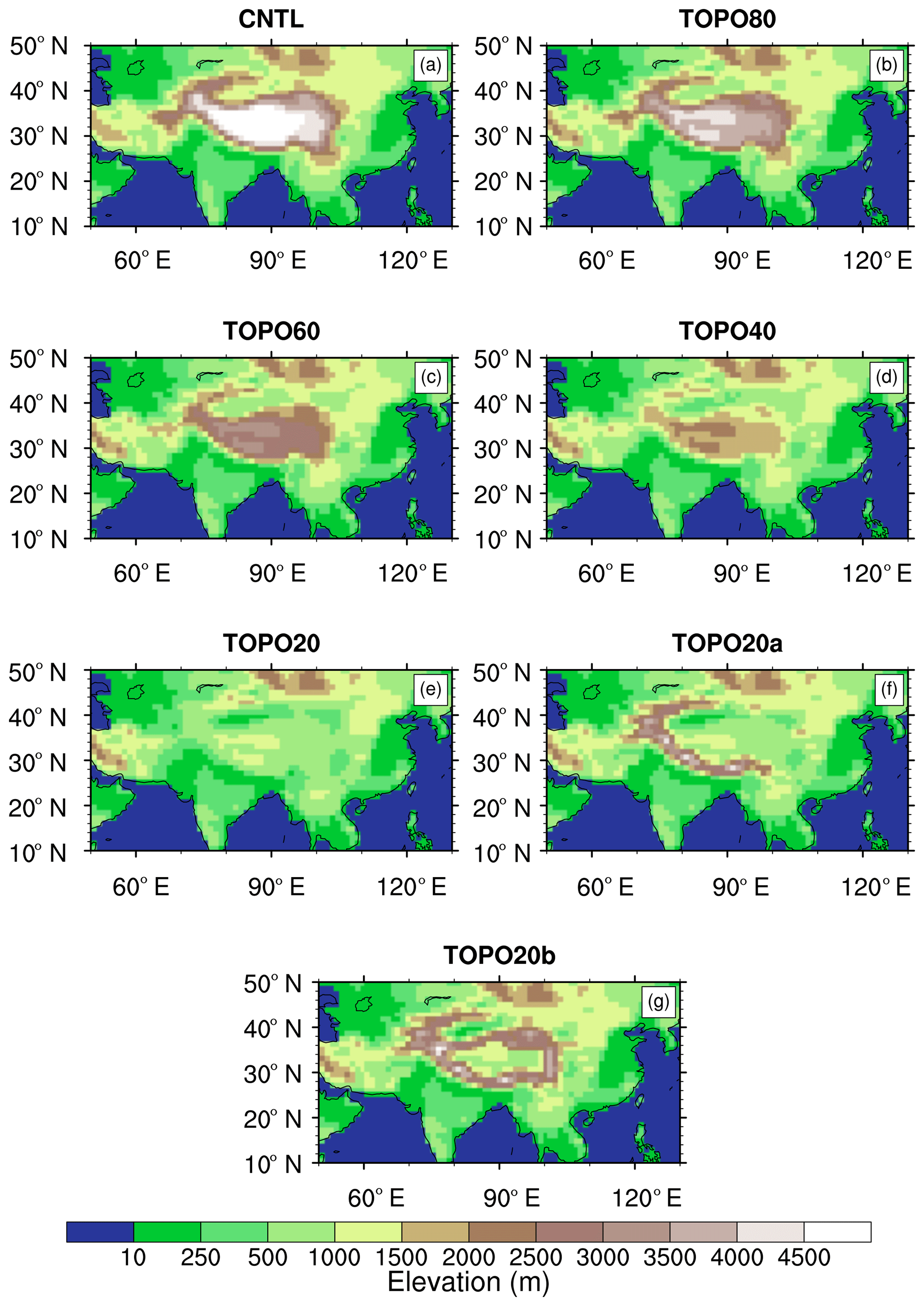
Figure 1 Surface elevations (m) prescribed in the ECHAM5 (a) CNTL, (b) TOPO80, (c) TOPO60, (d) TOPO40, (e) TOPO20, (f) TOPO20a, and (g) TOPO20b cases. Note that the CNTL simulation includes modern elevations. The names of the other cases (e.g., TOPO60) indicate the surface elevation of the Himalayan–Tibetan region relative to the modern elevation (e.g., 60 %). Cases TOPO2a and TOPO20b are modifications of the TOPO20 case (see Sect. 2).

Mean climate conditions today vary across the Himalaya; the western Himalaya is characterized by peak precipitation in winter and early spring, while the central Himalaya is dominated by the Indian summer monsoon (IM) and the eastern Himalayas are dominated by the East Asia summer monsoon (EASM) (Yao et al., 2013). Because of this heterogeneity, we separate the Himalayas into four distinct regions for analysis purposes: the western Himalayas; a transitional area between western and central Himalayas; central Himalayas; and eastern Himalayas (the transitional areas between the central and eastern Himalayas are excluded because the climate and isotopic signals are similar to the IM and EASM regions). The strength and pattern of precipitation and wind, and isotopic compositions in the two eastern-most transitional areas are similar to those in the IM and EASM in most cases. Thus, in the following we only present results for the western, transitional, IM, and EASM regions as shown in Fig. 2.

Figure 2 Topographic map (m) showing the Himalayan climate zones following Yao et al. (2013). Western, transitional, Indian summer monsoon (IM), and Eastern Asian summer monsoon (EASM) regions are marked. Transitional areas between the central and eastern Himalayas are excluded because the climate and isotopic signals are similar to the IM and EASM regions.

2.2 Rayleigh distillation

We developed an open-system, one-dimensional, altitude-dependent Rayleigh distillation model (RDM) in order to estimate decreases in δ¹⁸O_p due to Rayleigh distillation during ascent. The RDM tracks the isotopic composition of an air parcel as it ascends adiabatically from low to high altitude, becomes saturated, and loses condensate through precipitation. In the RDM, an air parcel cools at the dry adiabatic lapse rate before condensation and at the moist adiabatic lapse rate upon saturation (Rowley and Garzione, 2007). The RDM is run using terrain-following coordinates and is initialized with three different moisture sources: (1) fixed air temperature (T=20 ^∘C) and relative humidity (RH = 80 %); (2) local, summertime low-level T and RH from ECHAM5; and (3) fixed T=20 ^∘C and summertime RH from ECHAM5. In this way, we are able to quantify the influence due to total moisture source change – (1) minus (2) – and further decompose this influence into the changes in T – (3) minus (2) – or RH – (1) minus (3).

In order to estimate how much of the mass flux of ¹⁸O in total precipitation is contributed by the Rayleigh distillation process, we assumed that all large-scale precipitation, P_l, forms in response to stable upslope ascent and participates in Rayleigh distillation. We then estimated the isotopic flux of water undergoing Rayleigh distillation as follows:

$$\begin{array}{}\text{(1)}& {\displaystyle }{\displaystyle }\mathrm{RD}=\left({\displaystyle \frac{{{\mathit{\delta }}^{\mathrm{18}}\mathrm{O}}_{\mathrm{RDM}}}{\mathrm{1000}}}+\mathrm{1}\right)R_{\mathrm{vsmow}}\times P_{\mathrm{l}}\times {\mathit{\rho }}_{\mathrm{water}},\end{array}$$

where RD has units of g m⁻² h⁻¹, ρ_water (in g m⁻³) is the density of water, P_l (in m h⁻¹) is the large-scale precipitation rate, and δ¹⁸O_RDM is the isotopic composition simulated by the RDM at the same elevation as the grid points in Sect. 2.3 where the mass flux in total precipitation is estimated. Note that this estimation of RD stands for the upper limit of the contribution of RD, as not all large-scale precipitation is triggered by the Rayleigh distillation process.

To compare the relative importance of Rayleigh distillation with other isotopic fractionation processes in ECHAM, we quantify the change in upslope δ¹⁸O_p attributable to Rayleigh distillation. We do this by comparing the rate of upslope δ¹⁸O_p change (hereafter referred to as the δ¹⁸O_p lapse rates) in ECHAM with that estimated using the RDM. We define the δ¹⁸O_p lapse rate as the slope of the linear regression equation of precipitation-weighted δ¹⁸O_p regressed on elevation and use the coefficient of determination (R²) of this regression to evaluate the robustness of the δ¹⁸O_p–elevation relationship. We use a ratio of the δ¹⁸O_p lapse rate in ECHAM to that in the RDM (p_percent) to approximate the contribution of Rayleigh distillation to the ECHAM δ¹⁸O_p lapse rate. When R² and p_percent are both above 0.5 for a particular domain and elevation scenario, we consider that the ECHAM δ¹⁸O_p lapse rate agrees with the RDM δ¹⁸O_p lapse rate.

δ¹⁸O_p decreases as an air parcel travels inland. This continental effect may contribute to a significant portion of the decrease in δ¹⁸O_p over elevated regions in the low-elevation scenarios. To evaluate whether a strong δ¹⁸O_p–elevation relationship exists in low-elevation scenarios, we examine the ratio of the slope of δ¹⁸O_p regressed against latitude on the subcontinent to the south of the Himalayas to that on the Himalayan slope. This method accounts for the fact that δ¹⁸O_p changes with both latitude and elevation. A significant δ¹⁸O_p–elevation relationship is signified by a large ratio, indicating that Δδ¹⁸O_p with elevation is greater than that with latitude.

2.3 Quantifying effects through the mass flux of ¹⁸O

Mass fluxes of ¹⁸O are calculated to quantify the contribution of vapor mixing, surface recycling, and RDM to the ¹⁸O in total precipitation. Vapor mixing and surface recycling serve as the lateral and lower boundary sources of ¹⁸O in an air column, respectively, and total precipitation as the sink. Within this air column, sinks and sources of ¹⁸O in the air are assumed to compensate for one another to make the total mass of ¹⁸O in the air stable on climatological timescales, with the mass flux of ¹⁸O from vapor mixing and surface recycling balancing that from total precipitation. With this compensation of sources and sinks in mind, we calculated the flux of ¹⁸O due to vapor mixing, surface recycling, and total precipitation.

The vapor mixing between air masses is estimated as the advection of ¹⁸O in a vertical air column:

$$\begin{array}{}\text{(2)}& {\displaystyle }{\displaystyle \frac{\partial M{}^{\mathrm{18}}\mathrm{O}}{\partial t}}\sim \int -\stackrel{\mathrm{‾}}{V}\cdot \stackrel{\mathrm{‾}}{\mathrm{\nabla }}m{}^{\mathrm{18}}\mathrm{O}\mathrm{d}z,\end{array}$$

where M¹⁸O (g m⁻²) is the unit column-total mass of ¹⁸O in the air, $\stackrel{\mathrm{‾}}{V}$ (m h⁻¹) is the wind speed vector within a layer, m¹⁸O (g m⁻³) is the mass of ¹⁸O per m³ of air, and z (m) is elevation. Approximating the total mass of water by the amount of ¹⁶O, m¹⁸O is defined in terms of δ¹⁸O_c from Eq. (1) as

$$\begin{array}{}\text{(3)}& {\displaystyle }{\displaystyle }m{}^{\mathrm{18}}\mathrm{O}\approx q{\mathit{\rho }}_{\mathrm{air}}\left({\displaystyle \frac{{\mathit{\delta }}^{\mathrm{18}}\mathrm{O}}{\mathrm{1000}}}+\mathrm{1}\right)R_{\mathrm{vsmow}}.\end{array}$$

By substituting δ¹⁸O_c in Eq. (3) into Eq. (2), the final form of the total column-integrated vapor mixing (g m⁻² h⁻¹) is written as

$$\begin{array}{ll}{\displaystyle }VM& {\displaystyle }=\int -\stackrel{\mathrm{‾}}{V}\cdot \stackrel{\mathrm{‾}}{\mathrm{\nabla }}m{}^{\mathrm{18}}\mathrm{O}\mathrm{d}z=-\int \stackrel{\mathrm{‾}}{V}\\ \text{(4)}& {\displaystyle }& {\displaystyle }\cdot \stackrel{\mathrm{‾}}{\mathrm{\nabla }}\left[q{\mathit{\rho }}_{\mathrm{air}}\left({\displaystyle \frac{{\mathit{\delta }}^{\mathrm{18}}\mathrm{O}}{\mathrm{1000}}}+\mathrm{1}\right)R_{\mathrm{vsmow}}\right]{\mathit{\rho }}_{\mathrm{air}}\mathrm{d}z.\end{array}$$

Note that the centered-finite-difference method is used in discretizing the derivatives in Eq. (4). This method could potentially introduce errors in comparison to the spectral method used in the dynamical core of ECHAM5.

Recycling of surface water vapor transports ¹⁸O to the atmosphere from lower boundary. To estimate this contribution to ¹⁸O, the recycled mass flux (in g m⁻² h⁻¹) is calculated as follows:

$$\begin{array}{}\text{(5)}& {\displaystyle }{\displaystyle }\left({\displaystyle \frac{{\mathit{\delta }}^{\mathrm{18}}\mathrm{O}}{\mathrm{1000}}}+\mathrm{1}\right)R_{\mathrm{vsmow}}\times E\times {\mathit{\rho }}_{\mathrm{water}},\end{array}$$

where δ¹⁸O is the isotopic composition of the evaporated water and E (m h⁻¹) is the surface evaporation rate.

The mass flux of ¹⁸O in total precipitation is estimated in the following manner as per Eq. (3):

$$\begin{array}{}\text{(6)}& {\displaystyle }{\displaystyle }\left({\displaystyle \frac{{\mathit{\delta }}^{\mathrm{18}}\mathrm{O}}{\mathrm{1000}}}+\mathrm{1}\right)R_{\mathrm{vsmow}}\times P\times {\mathit{\rho }}_{\mathrm{water}},\end{array}$$

where δ¹⁸O is the isotopic composition of precipitation and P (m h⁻¹) is the precipitation rate.

Note that this method does not allow us to isolate within-column processes, including vertical mass exchanges through convective updrafts and downdrafts and through phase changes. We encourage future studies to isolate these within-column processes and establish how they evolve with topography.

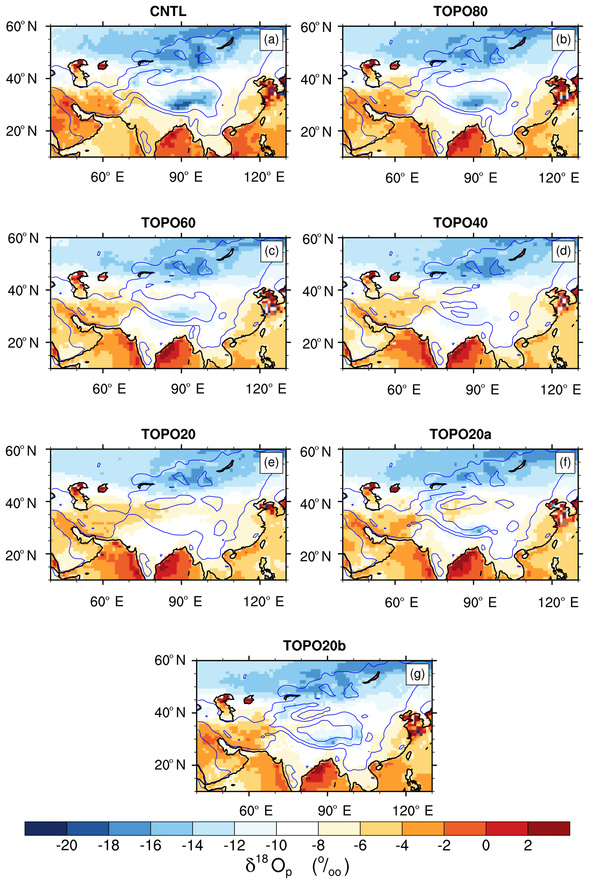
Figure 3 Mean-annual precipitation-weighted ECHAM δ¹⁸O_p (in ‰) for the (a) CNTL, (b) TOPO80, (c) TOPO60, (d) TOPO40, (e) TOPO20, (f) TOPO20a, and (g) TOPO20b cases. The blue contour lines represent 500 and 2000 m surface elevation contours.

3 Results

3.1 Model validation of ECHAM5-wiso

Under modern elevations, annual-mean precipitation-weighted δ¹⁸O_p decreases with elevation on the Himalayan slope, increases with latitude across the Tibetan Plateau (Figs. 3a, 4), and varies little (mostly within 2 ‰) on the northern Tibetan slope (36–40^∘ N; Fig. 4). Li et al. (2016) demonstrated that ECHAM5 simulates δ¹⁸O variations across the Himalayas and the Tibetan Plateau that are in reasonable agreement with observed precipitation and stream values (see Sect. 2). Consistent with stream water samples, the model captures a decrease in δ¹⁸O_p along a north–south transect across the Himalayas and an increase in δ¹⁸O_p on the Tibetan Plateau (see their Fig. 12d). The main discrepancy occurs in winter and spring on the northwestern Tibetan Plateau. Simulated δ¹⁸O_p is 4 ‰ greater than stream sample values along a cross section extending westward from 85^∘ E and centered on 30^∘ N. Li et al. (2016) attributed this mismatch to local factors, systematic model bias, and the influence of freshwater discharge from higher altitudes in the watershed.

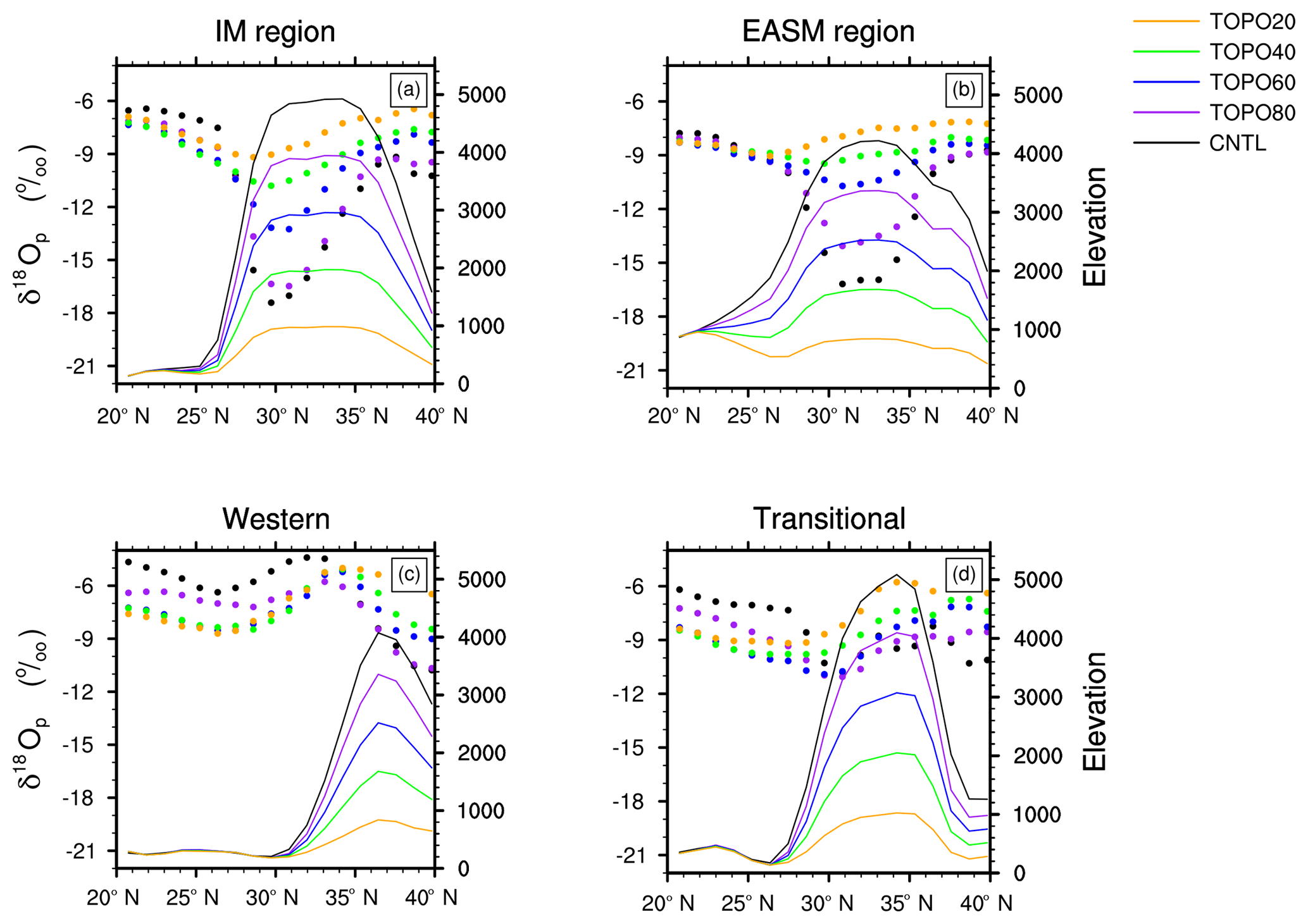
Figure 4 Annual-mean precipitation-weighted δ¹⁸O_p (filled circles) and surface elevations (lines) along latitudinal transects for the (a) IM, (b) EASM, (c) western, and (d) transitional regions. These values represent zonal-average values over the specific region.

We further compare ECHAM5 CNTL δ¹⁸O_p with the modern surface water isotope dataset reported in Li and Garzione (2017) (Fig. 5). Colocated ECHAM and water sample δ¹⁸O_p agree within 2 ‰ at 49.2 % of sites, and within 3 ‰ at 73.3 % of sites. Several discrepancies between simulated and observed δ¹⁸O_p exist. Firstly, ECHAM5 δ¹⁸O_p is lower than sampled δ¹⁸O_p over northwestern Tibet (35–37^∘ N, 80–85^∘ E). This mismatch could be associated with the higher relative humidity in ECHAM (Fig. S1 in the Supplement) than in the observations. This high relative humidity results in weaker evaporation both from land surface and below cloud-base, lowering δ¹⁸O in surface waters. Secondly, ECHAM5 δ¹⁸O_p is more depleted, by 2–5 ‰, over east-central Tibet (32–35^∘ N, 89–102^∘ E). The LMDZ-iso model shows a similar mismatch of 1–4 ‰ (Botsyun et al., 2016). In other regions of Tibet, simulated δ¹⁸O_p values in LMDZ-iso are very similar to those in ECHAM5, within 2 ‰ (Yao et al., 2013). There are two potential explanations for the mismatch from modern surface water over east-central Tibet. One possibility is that the sampled δ¹⁸O_p does not reflect mean climatic conditions. We note that the water samples from the east-central and northern Tibet regions were collected over a short 2-year span. This possibility is supported by the large interannual variability in δ¹⁸O_p (up to 9 ‰) in both ECHAM (Li et al., 2016) and precipitation samples spanning the period from 1986 to 1992 from GNIP (IAEA/WMO, 2017). The other source for the mismatch over east-central Tibet is the higher than observed precipitation simulated by ECHAM5, which can result in lower δ¹⁸O_p via the amount effect (as described in Sect. 3.6). The simulated summertime precipitation rate over east-central Tibet (32–35^∘ N, 89–102^∘ E) is 3.9 mm day⁻¹, which is higher than the 2.8 mm day⁻¹ from Climate Prediction Center (CPC) Merged Analysis of Precipitation (CMAP) datasets (for 1981–2010). This high precipitation is systematic and is also seen in other models, such as LMDZ-iso (Botsyun et al., 2016) and ECHAM4 (Battisti et al., 2014).

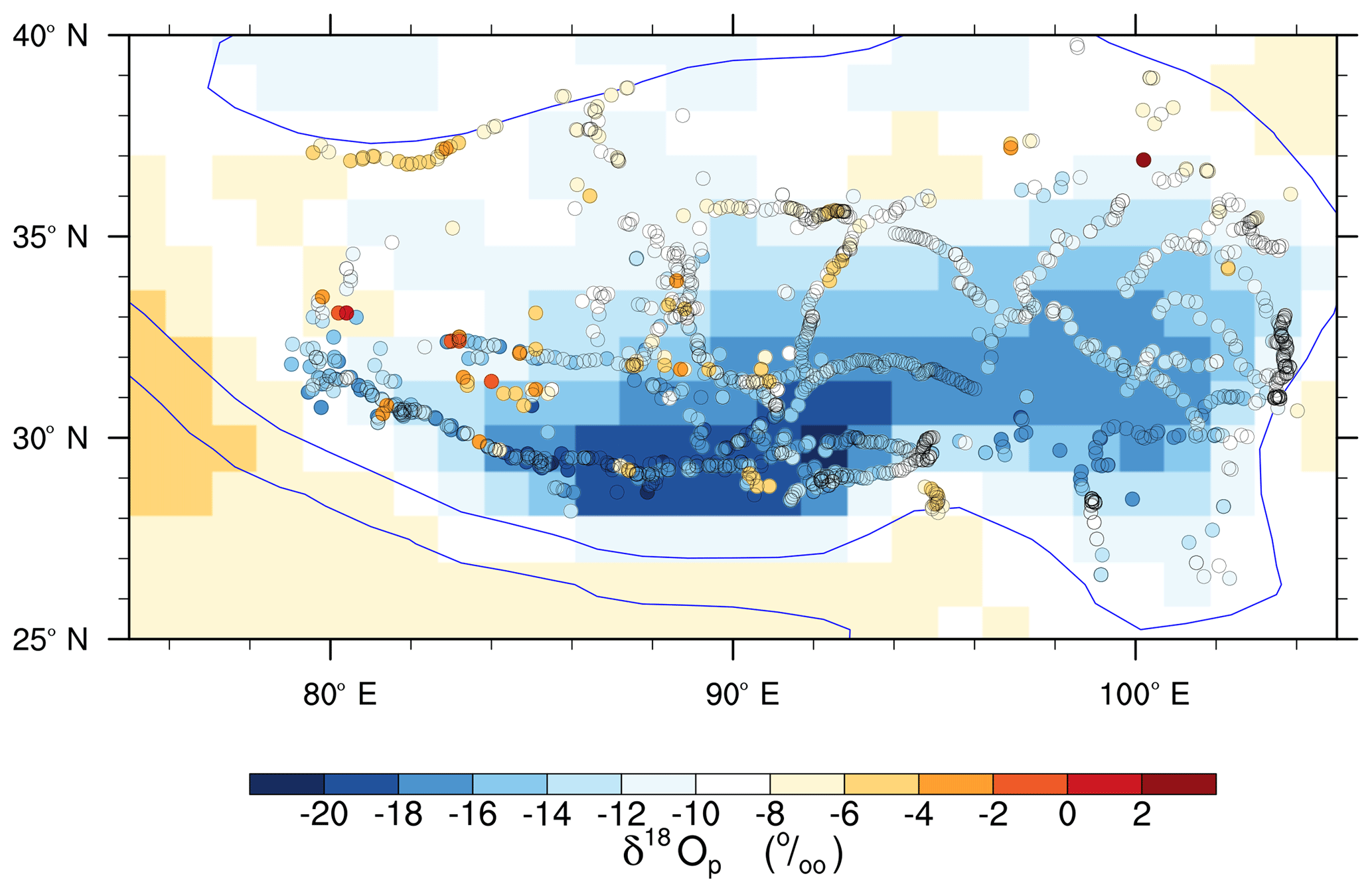
Figure 5 Comparison of annual-mean precipitation-weighted ECHAM δ¹⁸O_p (shaded) with precipitation and stream samples (circles) from Li and Garzione (2017).

3.2 Climate response to Tibetan–Himalayan surface elevation

Numerous modeling studies have found that lowering the height of the Tibetan Plateau influences regional temperature, wind, precipitation, and relative humidity (e.g, Kitoh, 2004; Jiang et al., 2008). In this section, we describe regional climate changes on the western Himalayan slope, the Tibetan Plateau, the IM region, and the EASM region, which occur as high elevations are lowered.

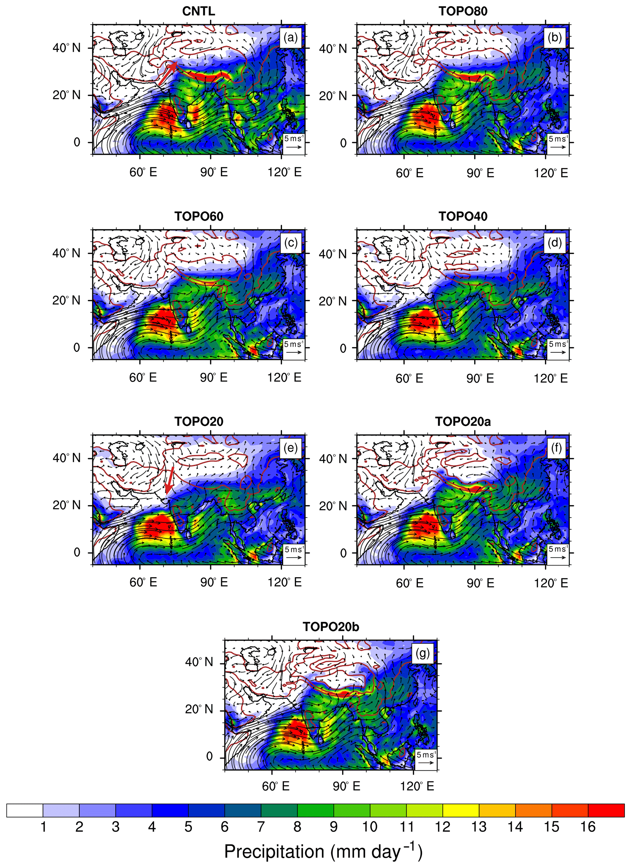
Figure 6 Summer (June–July–August) low-level (850 hPa) wind (arrows) and precipitation (shaded) for the (a) CNTL, (b) TOPO80, (c) TOPO60, (d) TOPO40, (e) TOPO20, (f) TOPO20a, and (g) TOPO20b cases. Brown contour lines represent 500 and 2000 m surface elevation contours in the Tibetan region. The red arrows on the western Himalayan slope in (a) and (e) show the wind direction reversal from CNTL to TOPO20.

Under modern conditions, near-surface temperatures in the Tibetan–Himalayan region vary with elevation following a moist adiabatic lapse rate (∼5 ^∘C km⁻¹; Fig. S2) and range from >30 ^∘C on the Indian subcontinent at the foot of the Himalayas to <10 ^∘C across the Tibetan Plateau (Fig. S3a). Lowering elevations in our experiments causes near-surface temperatures across the Tibetan–Himalayan region to increase (Fig. S3b–g) at approximately the lapse rate for the CNTL case. As a result, temperature lapse rates vary little among elevation scenarios, for instance, ranging from 4.9 to 5.4 ^∘C km⁻¹ in the IM region (Fig. 1).

Wind patterns, precipitation, and RH respond dramatically to reductions in elevation. These changes vary across regions. On the western Himalayan slope, wind directions nearly reverse with southerly winds in the high-elevation scenarios switching to northwesterly winds in low-elevation scenarios (Fig. 6). This wind reversal results in the transport of arid air from the north, which lowers total-column relative humidity by ∼40 %. With this substantial decrease in RH, summer precipitation decreases from ∼3 mm day⁻¹ in the CNTL to ∼0.1 mm day⁻¹ on the western Himalayan slope in TOPO20. A similar decrease in RH, by ∼20 % from the CNTL to TOPO20, is simulated on the Tibetan Plateau. Accompanying this reduction in RH, precipitation on the Tibetan Plateau decreases from ∼4 mm day⁻¹ in the CNTL to ∼1 mm day⁻¹ in TOPO20. This reduction in Tibetan Plateau precipitation is linked to a weakening of the Asian monsoonal systems and moisture delivery through monsoonal winds.

The responses in the monsoonal regions are somewhat different from those on the western slope of the Himalayas and the Tibetan Plateau. A reduction in surface elevation (from CNTL to TOPO20; Fig. 1) leads to a weakening of the IM, as indicated by a slowing of summer southwesterly winds over the Bay of Bengal and the Arabian Sea and a decrease in summer precipitation (by more than 20 mm day⁻¹ in ECHAM) along the central Himalayas (Fig. 6). IM weakening is also demonstrated by the WSI1 monsoon index (Fig. 7, following Wang and Fan, 1999), which is defined by the vertical wind shear between the lower (850 hPa) and upper (200 hPa) troposphere in the region (5–20^∘ N, 40–80^∘ E) during summer. Monthly WSI1 index values (not shown) indicate that the Indian monsoon persists through all elevation scenarios, although summertime WSI1 (Fig. 7) shows that it weakens abruptly once elevations are reduced to between 40 % and 60 % of modern values, a threshold reported in previous modeling studies (e.g., Abe et al., 2003). As a result of IM weakening, total-column average RH decreases from >90 % in CNTL to 70 % in TOPO20 and summer precipitation decreases from >16 mm day⁻¹ in CNTL to ∼6 mm day⁻¹ in TOPO20.

ECHAM5 captures a similar threshold behavior in monsoon activity in the EASM region. With lowering of the Himalayan front to 40 % of its modern elevations, the broad humid belt that characterizes central China in high-elevation scenarios (CNTL, TOPO80, TOPO60, TOPO20a, and TOPO20b) shifts southward, resulting in an expanded arid belt in the region (in TOPO40 and TOPO20). This shift in precipitation is associated with a southward retreat of the southwesterly monsoonal winds that penetrate much of eastern Asia (Fig. 6d, e).

3.3 Climate response to Himalayan surface elevation

ECHAM5 experiments TOPO20a and TOPO20b isolate the influence of Himalayan elevations on the regional climate. These experiments generally indicate that the Himalayas, rather than the Tibetan Plateau, govern regional precipitation and circulation patterns. The IM and EASM are strong in both TOPO20a and TOPO20b. The IM is shown by strong low-level wind over the Arabian Sea and heavy precipitation across both the Indian subcontinent and the central Himalayas in TOPO20a and TOPO20b (Fig. 6f, g). Likewise, the EASM in these simulations is similar to that in the CNTL as indicated by heavy precipitation to the north of the Yangtze River and southerly winds penetrating central China (Fig. 6f, g).

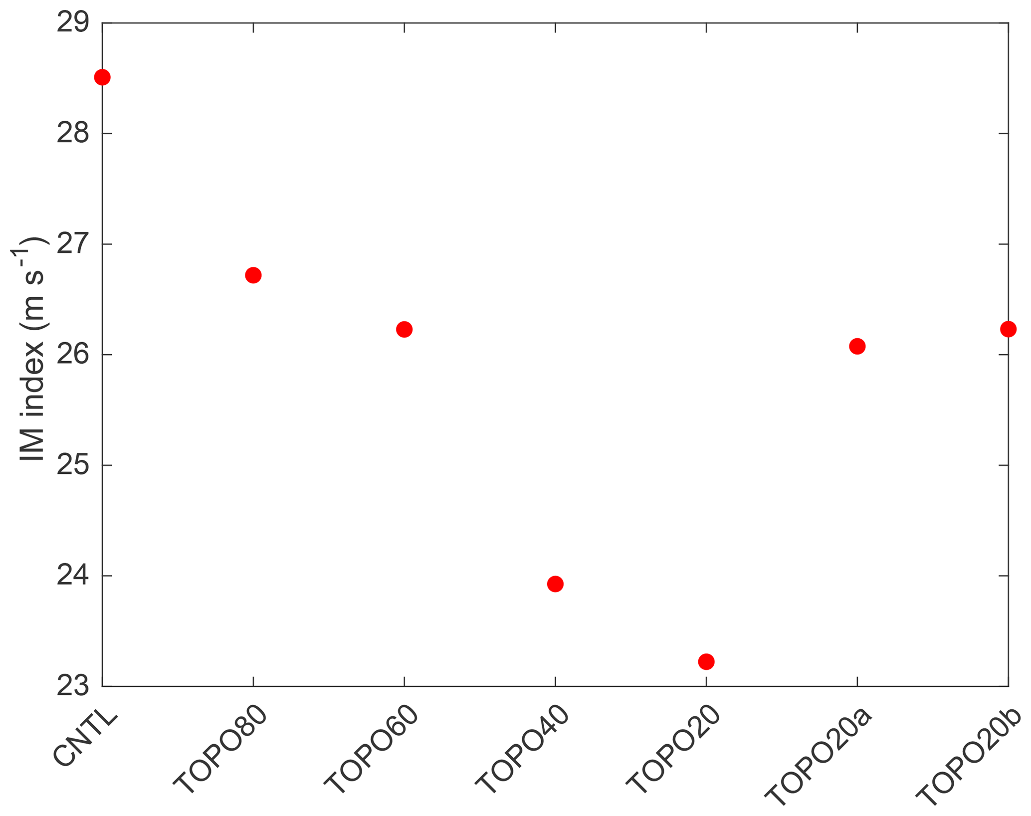
Figure 7 Indian summer monsoon (June–July–August) index, WSI1, calculated as the vertical wind shear between the lower (850 hPa) and upper (200 hPa) troposphere in the region (5–20^∘ N, 40–80^∘ E).

To further elucidate the contribution of the Himalaya to monsoonal dynamics, we calculated the equivalent potential temperature (Fig. S4), which is commonly used to denote the location of monsoonal heating for the Indian monsoon. In TOPO20a and TOPO20b, the equivalent potential temperature maxima are reduced but in a similar location to the CNTL case, supporting our conclusion that the Himalayas are the dominant driver of the IM. When the Himalayas are lowered, monsoonal heating decreases and the locus shifts southeastward as cold, dry extratropical air moves southward and mixes with warm, humid subcontinental air, consistent with the results in Boos (2015), although the extent of the shift is smaller in ECHAM5.

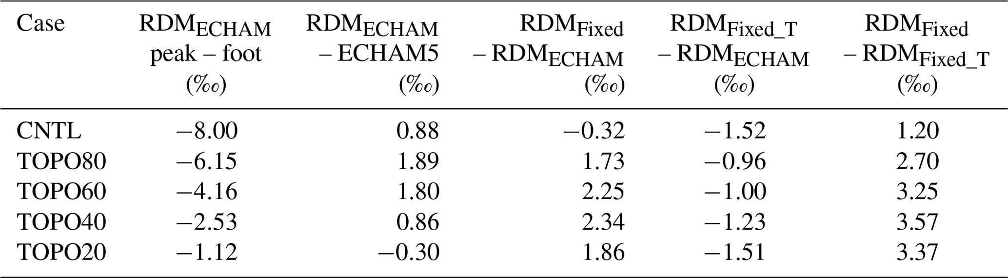
Table 1 Contribution of physical processes to annual-mean precipitation-weighted δ¹⁸O_p (all units in ‰) averaged over monsoonal regions (IM and EASM). In the table, RDM_ECHAM represents the RDM initiated using the moisture sources (i.e., air temperature and relative humidity) from ECHAM5; RDM_Fixed is the δ¹⁸O_p simulated by a RDM initiated with fixed moisture source of T=20 ^∘C and RH = 80 %; and RDM_{Fixed_T} is initiated with fixed T=20 ^∘C and ECHAM RH (refer to Sect. 2.2 for more details on the three different moisture sources). All columns show values averaged from mountain foot to mountain peak, except for the second column that shows the difference in δ¹⁸O_p between mountain peak and foot as simulated by RDM_ECHAM.

In contrast to this well established mechanism for the Indian monsoon, the mechanism for the southward shift of the EASM is not well understood. Uplift of the Himalaya–Tibet orogen (Guo et al., 2008; Liu et al., 2017), the retreat of the Paratethys (Guo et al., 2008), and forcing by atmospheric pCO₂ (Licht et al., 2014; Caves Rugenstein and Chamberlain, 2018) have been proposed as possible factors triggering this southward shift, although the timing for the shift is highly debated from the Eocene to the early Miocene. Our simulation of a strong EASM over central China in both TOPO20a and TOPO20b suggests that uplift of the central and western Himalaya would have been capable of forcing this southward shift.

3.4 Moisture source influence on RDM δ¹⁸O_p

Under lower elevation scenarios, δ¹⁸O_p values increase relative to the modern elevation scenario both on the Himalayas and the Tibetan Plateau (Fig. 4). The rate of change of δ¹⁸O_p with elevation and latitude decreases substantially in the monsoonal regions as Tibetan–Himalayan elevations are reduced (Fig. 4a, b).

The oxygen isotope compositions of precipitation on mountain slopes are traditionally assumed to systematically decrease in response to adiabatic cooling, condensation, and rainout of ascending air parcels, a process described by Rayleigh distillation and the basis for the application of δ¹⁸O_p paleoaltimetry. In this section, we evaluate the degree to which Rayleigh distillation accounts for upslope decreases in δ¹⁸O_p by comparing RDM to ECHAM δ¹⁸O_p in four separate regions (Fig. 2). Note that the northern Tibetan slope is excluded here because most of the northerly air is diverted rather than being forced to ascend (Fig. 6).

For each of the four regions, we initialize the RDM with both fixed moisture sources (with initial T=20 ^∘C and RH = 80 %) as in paleoaltimetry studies and with ECHAM moisture sources (with a T and RH that vary by region and case). The δ¹⁸O_p predicted by the RDM using each moisture source is shown in Figs. 8 and 9 (red diamonds versus black circles). With ECHAM-derived T and RH, the RDM δ¹⁸O_p values are close to those simulated by ECHAM5 in all elevation scenarios (Figs. 8, 9; Table 1, third column). RDM δ¹⁸O_p with ECHAM-derived moisture is 0–2 ‰ less than that with fixed T and ECHAM RH (Table 1, fourth column), except in the CNTL scenario where the two RDM δ¹⁸O_p are very close. The lower δ¹⁸O_p is due to the fact that the RH of the initial air parcel is lower in ECHAM than in the prescribed case (Fig. S1). The impact of moisture source differences on δ¹⁸O_p is further decomposed in Table 1 to estimate the contributions of adiabatic temperature versus RH changes. As seen in Table 3, the effect of adiabatic temperature changes is consistently small ($\sim -\mathrm{1}$ ‰) across all elevation scenarios, reflecting the fact that temperature lapse rates vary little among elevation scenarios (Fig. S2). In contrast, as the initial RH decreases with the lowering of elevation, ECHAM-sourced δ¹⁸O_p is lowered by as much as 3.5 ‰ (Table 1, last column). In summary, these results demonstrate that elevation-related changes in moisture source characteristics substantially impact RDM δ¹⁸O_p estimates.

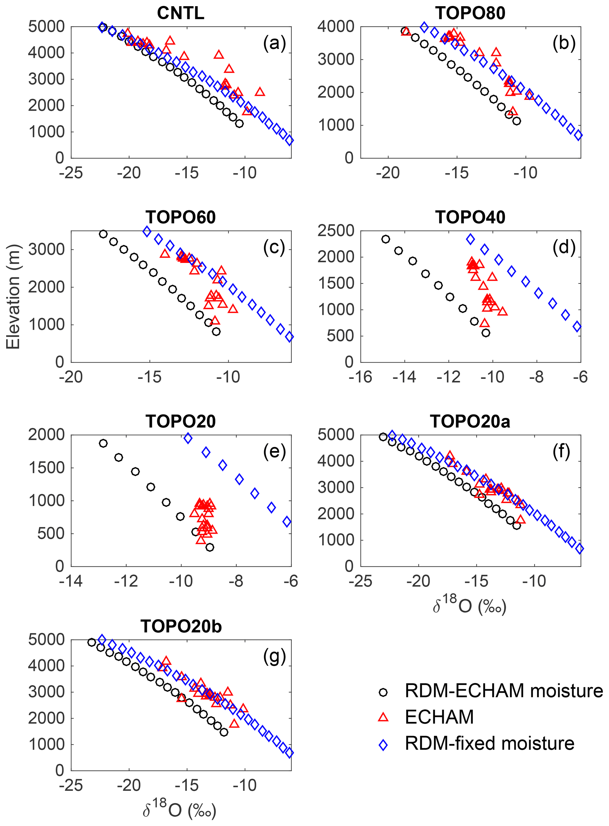
Figure 8 δ¹⁸O_p (‰) versus elevation (m) for the Indian summer monsoon (ISM) region of the southern Himalayan flank as simulated by ECHAM5 (blue triangle, annual-mean precipitation-weighted), RDM initiated with ECHAM5 summertime moisture sources (black circle), and RDM initiated with fixed moisture sources of T=20 ^∘C and RH = 80 % (red diamond) for the (a) CNTL, (b) TOPO80, (c) TOPO60, (d) TOPO40, (e) TOPO20, (f) TOPO20a, and (g) TOPO20b cases.

3.5 Performance of ECHAM-sourced Rayleigh distillation in the Himalayas

Our estimates using an RDM implicitly assume that Rayleigh distillation is the dominant process controlling the δ¹⁸O_p–elevation relationship. To test this assumption, we compare ECHAM-sourced RDM δ¹⁸O_p and ECHAM5 δ¹⁸O_p.

Table 2 Summary of the comparison between ECHAM and RDM δ¹⁸O_p lapse rates under different topographic scenarios in different climate regions. Regions and scenarios with a high R² and p_percent are marked with an “X” indicating the existence of a significant δ¹⁸O_p–elevation relationship (see methods in Sect. 2.2 for definitions of R² and p_percent).

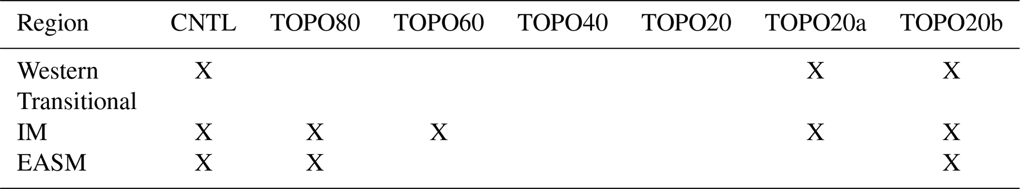
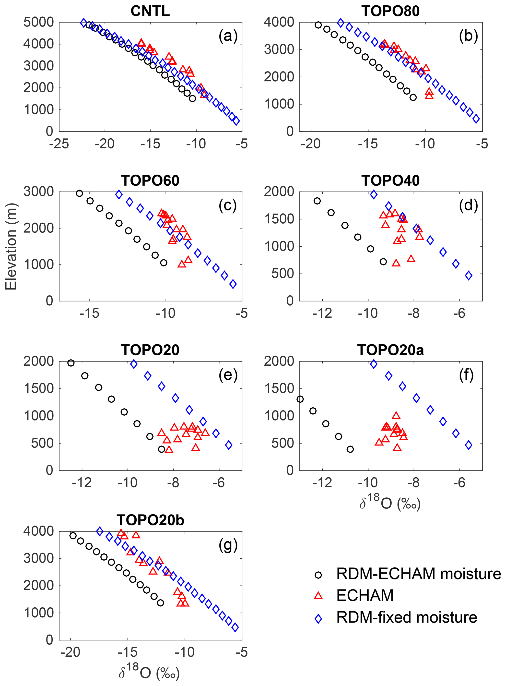
Figure 9 Same as in Fig. 7 but for the East Asian summer monsoon (EASM) region of the southern Himalayan flank.

Decreases in δ¹⁸O_p with elevation in ECHAM and the RDM generally agree under high-Himalaya scenarios and are consistent with modern observations (Table 2). Under modern topographic scenarios for the western Himalaya (Fig. S5) and the monsoonal regions (Figs. 8, 9), R² and p_percent values are greater than 0.77 and 0.51, respectively, indicating that RDM and ECHAM δ¹⁸O_p match well. R² and p_percent values are similarly high, above 0.68 and 0.53, respectively, for the western Himalaya and the monsoonal regions in the high-Himalaya scenarios (TOPO80, TOPO60, TOPO20a, and TOPO20b in the IM region; TOPO80 and TOPO20b in the EASM region) again indicating a good match between ECHAM and RDM δ¹⁸O_p and suggesting that Rayleigh distillation drives isotopic compositions in these regions.

In other regions and under low-elevation scenarios, however, the comparison between RDM and ECHAM δ¹⁸O_p is poor (Table 2). For instance, on the western Himalayas, in the TOPO80 case (Fig. S5), the lapse rate of ECHAM δ¹⁸O_p is much smaller than the lapse rate predicted by the RDM (Fig. S5), as shown by the p_percent values of less than 0.15. Under even lower elevation scenarios (TOPO60, TOPO40, and TOPO20), orographic precipitation is not triggered over the Himalayas (Fig. S4c–e), making the RDM an unsuitable representation of precipitation processes. In the transitional region, the δ¹⁸O_p can vary by more than 5 ‰ at a specific elevation under all elevation scenarios (Fig. S6). This large spread is represented by a low R² value of 0.12 for the CNTL case, and even lower values (less than 0.10) for other topographic scenarios. In TOPO40 and TOPO20, ECHAM δ¹⁸O_p shows little relationship with elevation (Fig. 4d).

In the monsoonal regions, the relationship between ECHAM5 δ¹⁸O_p and elevation is weak in low-elevation scenarios (Table 2, Fig. 4) and compares poorly with the RDM. In the IM region, p_percent values for the TOPO40 and TOPO20 are less than 0.29. In the EASM region, ECHAM5 δ¹⁸O_p is higher than RDM δ¹⁸O_p (Figs. 8, 9) in the TOPO60 scenario and the agreement is low (with a p_percent value of 0.31). Under even lower elevation scenarios (TOPO40 and TOPO20), ECHAM δ¹⁸O_p shows no relationship with elevation (Table 2, Fig. 4b) and also compares poorly with the RDM (with a p_percent value less than 0.29).

Among the high-Himalaya–low-Tibet cases (TOPO20a and TOPO20b), RDM and ECHAM δ¹⁸O_p match well in the IM region. The match is similarly good for TOPO20b in the EASM region. However, in the case with a low eastern flank (TOPO20a), the comparison is poor with an R² of 0.006 and a p_percent of −0.05.

Figure 10 Summertime mass flux of ¹⁸O (g m⁻² h⁻¹) for the (a) western Himalayas, (b) the transitional, (c) the IM, and (d) the EASM regions. Sources (positive values) and sinks (negative values) balance within 20 % or 0.1 g m⁻² h⁻¹ for fluxes that are close to zero. (Small errors in the net balance arise due to the centered-finite-difference method used to calculate derivatives in the advection terms.) Note that the largest source/sink varies by region and with elevation. Local convection and surface recycling are the dominant respective source and sink of ¹⁸O in the western Himalayas and under low-elevation scenarios, while Rayleigh distillation and vapor mixing dominate in high-elevation scenarios in the monsoonal and transitional regions.

3.6 Factors influencing the δ¹⁸O_p–elevation relationship on the Himalayan slope

As shown in Sect. 3.5, Rayleigh distillation cannot explain δ¹⁸O_p variations with elevation for most regions in the reduced elevation (TOPO40 and TOPO20) scenarios and in many regions under higher elevation scenarios (TOPO80 and TOPO60). To understand the factors influencing δ¹⁸O_p, we quantify the mass fluxes of ¹⁸O (Fig. 10), distinguishing the processes that increase the mass flux of ¹⁸O of the column (mixing and surface recycling) from those that decrease it (Rayleigh distillation and convective rainfall). Note that this method of taking the vertical column as a whole does not isolate the processes occurring within the air column (e.g., sub-cloud reevaporation, vertical advection, and mixing); this limitation does not impact our ability to identify the contributions of Rayleigh distillation and local processes. The results from this method yield very different contributions on the western slope from those in other regions; thus, the western Himalayas are reported separately.

On the western Himalayas, local surface recycling and convective rainfall contribute substantially to the total mass flux of ¹⁸O_p in the highest elevation scenarios (Fig. 10a). The contributions from these processes account for the poor match between RDM and ECHAM δ¹⁸O_p in this region. In the TOPO20a and TOPO20b scenarios, enhanced transport of enriched vapor from the south (see Fig. S7, 1 of 42 trajectories in CNTL versus 11 and 13 of 42 in TOPO20a and TOPO20b, respectively) increases the contribution from vapor mixing.

Table 3 The isotopic contribution (in ‰) due to summertime sub-cloud reevaporation and surface recycling on the Tibetan Plateau for different elevation scenarios.

In the monsoonal regions and the transitional region, vapor mixing is the predominant source of ¹⁸O under high-elevation scenarios and reflects the advection of ¹⁸O-enriched vapor from the Arabian Sea and the Bay of Bengal. This mass flux of vapor mixing decreases substantially with a reduction in elevation, whereas the mass flux of surface recycling remains approximately constant in all elevation scenarios. As a result, surface recycling is as or more important than mixing as a source of ¹⁸O under low-elevation scenarios (Fig. 10c, d). This change in the relative importance of the two sources represents an increase in the importance of local versus remote sources as monsoon strength weakens under low-elevation scenarios.

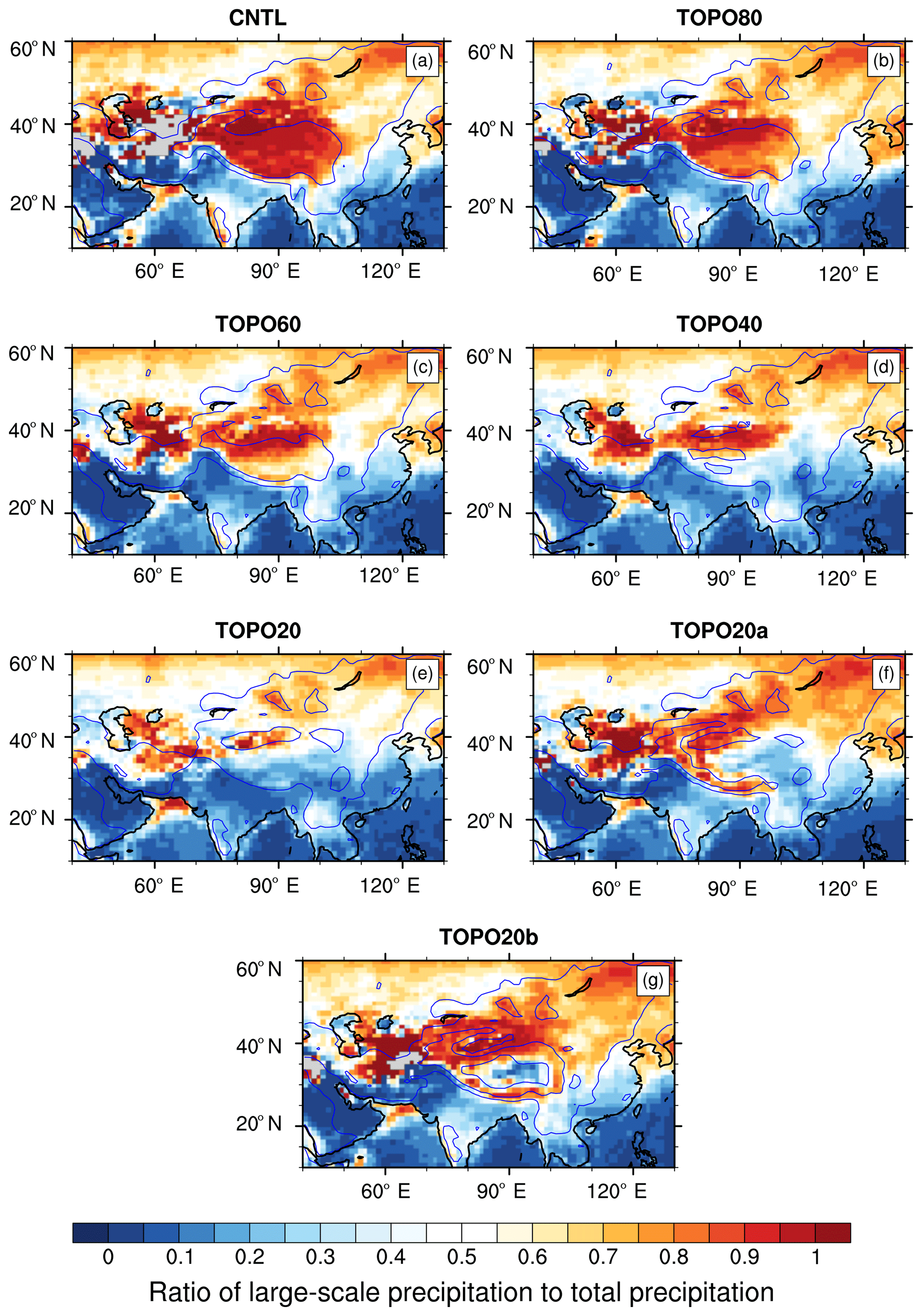
Figure 11 Ratio of summer large-scale to total precipitation rate in the (a) CNTL, (b) TOPO80, (c) TOPO60, (d) TOPO40, (e) TOPO20, (f) TOPO20a, and (g) TOPO20b cases. Blue lines mark the 500 and 2000 m elevation contours in each case. In the Himalayas, this ratio decreases when mountain elevations are reduced. As a result, large-scale precipitation is dominant in high-elevation scenarios, but not in low-elevation scenarios.

In high-elevation scenarios, Rayleigh distillation acts as the dominant sink of ¹⁸O in the monsoonal regions causing δ¹⁸O to decrease markedly with elevation (Fig. 10c, d). Under reduced elevation scenarios, the absolute mass flux from Rayleigh distillation decreases, as large-scale precipitation due to stable upslope ascent decreases and convective precipitation increases (Fig. 11). With reduced elevation, the percentage of large-scale precipitation to total precipitation falls from 86 % to 18 % in the transitional region, from 93 % to 18 % in the IM region, and from 80 % to 15 % in the EASM region, mirroring the decrease in the mass contribution of Rayleigh distillation, which falls from 85 % to 11 % in the transitional region, from 93 % to 22 % in the IM region, and from 80 % to 18 % in the EASM region. As a result of the reduction in (large-scale) precipitation by stable upslope ascent, convective precipitation becomes the largest ¹⁸O sink in TOPO20 and TOPO40 in both the transitional region and the IM region, and in TOPO60, TOPO40, TOPO20, and TOPO20a in the EASM region. These are also the scenarios that exhibited a poor match between RDM δ¹⁸O_p and ECHAM δ¹⁸O_p (Sect. 3.5). The increase in convective rainfall in these cases leads to greater kinetic fractionation through the sub-cloud evaporation of falling rain, which is only partially equilibrated with the surrounding vapor (see Sect. 2.1), and an enrichment in the isotopic composition of rain. The RDM does not capture this enrichment because it does not include sub-cloud evaporation. A similar reduction in large-scale precipitation with a reduction in elevation is also captured in the Andes region (Insel et al., 2009) and is associated with a decrease in the rate of change of δ¹⁸O_p with elevation.

Note that, although Rayleigh distillation is the primary sink under high-elevation scenarios, RDM δ¹⁸O_p does not match ECHAM δ¹⁸O_p well in the transitional region because of the large spread in ECHAM δ¹⁸O_p (Fig. S6). This spread is due to the bifurcated sources from northwest India (relatively enriched) and the Bay of Bengal (relatively depleted), as air parcels follow separate trajectories before mixing at the peak (Fig. S7).

In summary, the mismatch between RDM and ECHAM δ¹⁸O_p is caused by a weakening of Rayleigh distillation under low-elevation scenarios, triggered by a reduction in large-scale precipitation.

3.7 δ¹⁸O_p–latitude relationship on the Tibetan Plateau

In contrast to δ¹⁸O_p on the Himalayas, δ¹⁸O_p on the Tibetan Plateau increases linearly with latitude. It has been proposed that past δ¹⁸O_p, reconstructed from the isotopic analyses of ancient soil and lake carbonates, could provide information about past elevations on the Tibetan Plateau after removing the modern meridional δ¹⁸O_p gradient (Bershaw et al., 2012). This proposal is problematic because the meridional δ¹⁸O_p gradient and the processes that set this gradient on the Tibetan Plateau are poorly understood today and were likely different in the past in ways that are not known.

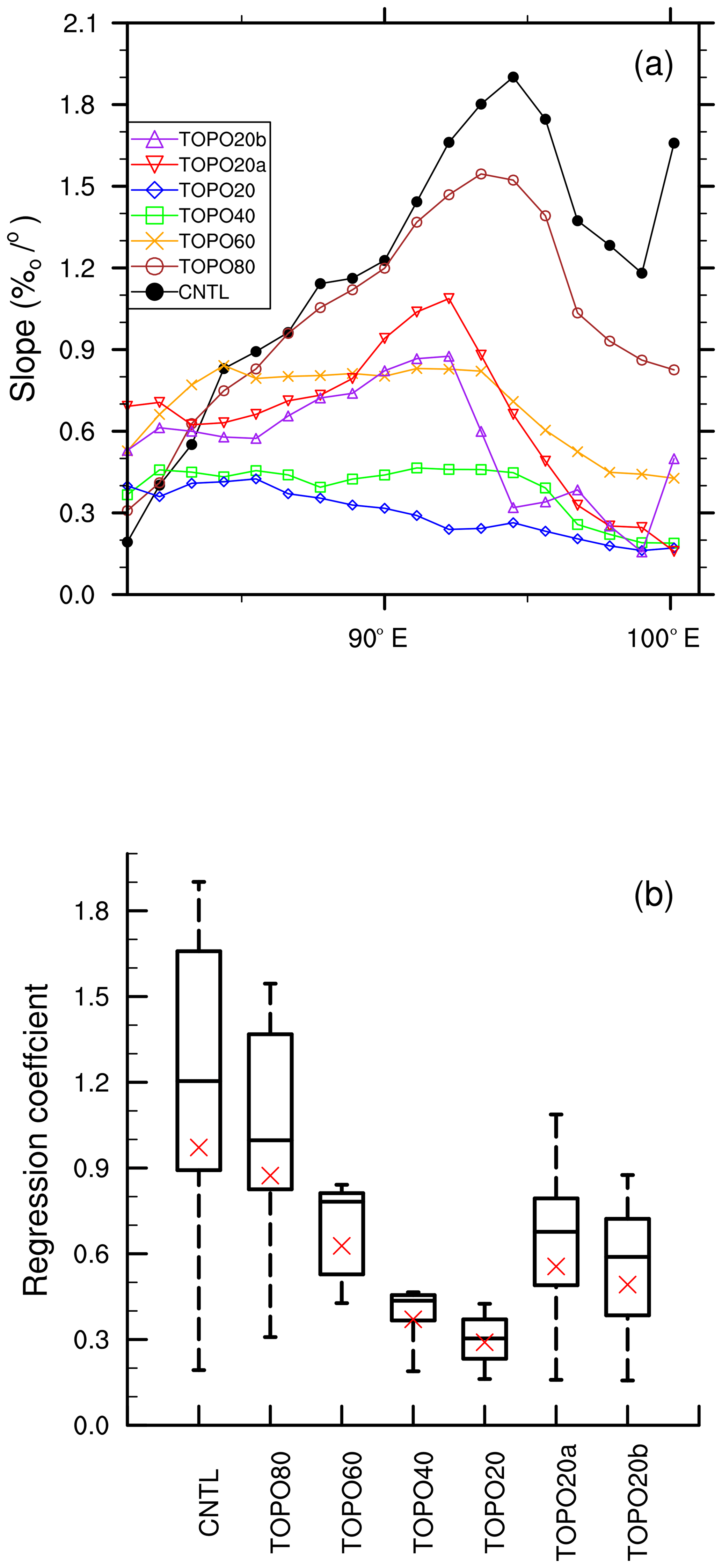
Figure 12 (a) The slope (in ‰ ^∘−1) of the linear regression of annual-mean precipitation-weighted δ¹⁸O_p on latitude from ECHAM5 output, used as an approximation for the meridional gradient of δ¹⁸O_p. (b) The box plot shows the variability of the meridional gradient of δ¹⁸O_p. The red “x” indicates mean values for each scenario, calculated by regressing longitudinally averaged δ¹⁸O_p across the Tibetan Plateau on latitude. Box plots show minimum, maximum, median, and quartile values.

Tibetan Plateau meridional δ¹⁸O_p gradients simulated by ECHAM5 under modern and reduced elevation scenarios are shown in Fig. 12. The average meridional gradient in the CNTL is 0.95 ‰ ^∘−1, which is very close to the observed gradient of 1.09 ‰ ^∘−1 (Li and Garzione, 2017). Three features of the latitudinal δ¹⁸O_p gradients are notable. Firstly, the gradient varies with longitude (Fig 12a, b) and variations are larger in high-elevation cases (e.g., from 1.90 to 0.20 ‰ ^∘−1 in the CNTL). Secondly, a linear fit is generally good with a high coefficient of determination (R²>0.8) east of 85^∘ W for all cases except TOPO20a and TOPO20b (Fig. S8). The high goodness of fit indicates a robust δ¹⁸O_p–latitude relationship for the cases with uniform reductions in topography. The poor fit in TOPO20a and TOPO20b is due to the larger variations in elevation across the Tibetan Plateau. In these two cases, dry conditions (Fig. S1) on the steep leeward side of the Himalayas favor strong below cloud-base reevaporation, which increase local latitudinal δ¹⁸O_p gradients. Lastly, in cases with a uniform lowering of topography, the median meridional gradient (Fig. 12b) decreases almost linearly with reductions from 100 % to 60 % of modern topography, changes more abruptly between 60 % and 40 %, and varies little once the topography is lowered below the monsoon threshold in TOPO40 and TOPO20.

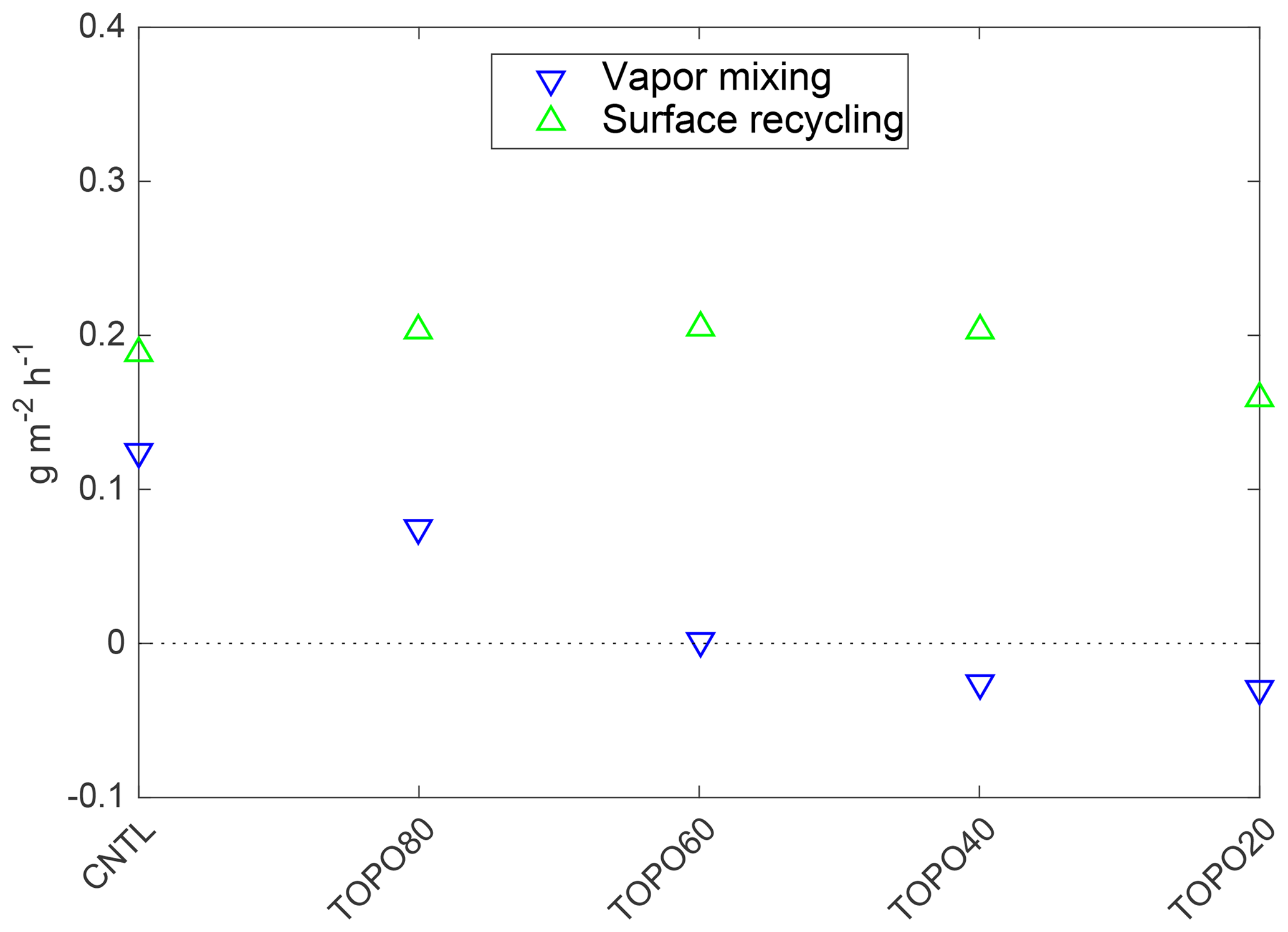
Figure 13 The mass flux of ¹⁸O (g m⁻² h⁻¹) from summertime (June–July–August) vapor mixing and surface recycling on the Tibetan Plateau. Note that the positive (negative) values indicate sources (sinks) of ¹⁸O. Surface recycling is the largest source of ¹⁸O under all elevation scenarios. Vapor mixing is secondary as a source in high-elevation scenarios and becomes a sink in low-elevation scenarios.

The modern latitudinal δ¹⁸O_p gradient on the Tibetan Plateau has been attributed to both surface recycling and sub-cloud reevaporation. Surface recycling increases δ¹⁸O_p by adding more enriched vapor from the land surface, while sub-cloud evaporation enriches ¹⁸O in precipitation by partial evaporation of falling raindrops in an unsaturated air column. To understand the cause of the decline in the meridional δ¹⁸O_p gradient, we quantified both the sources of ¹⁸O (surface recycling and vapor mixing) and the isotopic contribution due to sub-cloud reevaporation. Sub-cloud evaporation is quantified separately because this effect is contained in but cannot be isolated from the sources of ¹⁸O.

Surface recycling is the primary source of ¹⁸O on the Tibetan Plateau with largely consistent contributions under all elevation scenarios (Fig. 13). The mass flux of ¹⁸O due to vapor mixing is small and becomes a sink in low-elevation scenarios, as there are increasingly more depleted sources from the south in these scenarios (e.g., 17 out of 42 in the CNTL versus 30 out of 42 in TOPO20 for one location – 33^∘ N, 90^∘ E). To further quantify the contribution of surface recycling to total precipitation, we subtracted δ¹⁸O in precipitation from δ¹⁸O in recycled vapor and normalized by the amount of precipitation and recycled vapor as in the following equation:

$$\begin{array}{}\text{(7)}& {\displaystyle }{\displaystyle }\left({{\mathit{\delta }}^{\mathrm{18}}\mathrm{O}}_{\mathrm{s}}-{{\mathit{\delta }}^{\mathrm{18}}\mathrm{O}}_{\mathrm{p}}\right)\times E/P\times {\mathit{\rho }}_{\mathrm{water}},\end{array}$$

where δ¹⁸O_p is the isotopic composition in precipitation, δ¹⁸O_s is the condensate of recycled vapor, E (m h⁻¹) is the surface evaporation rate, and P (m h⁻¹) is the total precipitation rate. Results from Eq. (7) show that δ¹⁸O of surface recycling contributes less than 0.1 ‰ in the CNTL and slightly more (−2.67 ‰) in TOPO20 (Table 3). The overall small contribution from surface recycling in ECHAM5 is due to the fact that δ¹⁸O values in soil are similar to those in precipitation (Fig. S9). This small contribution grows in low-elevation scenarios due to the increased fraction of evaporated vapor to total precipitation (Fig. S10). Nonetheless, surface recycling plays a secondary role in decreasing the meridional δ¹⁸O_p gradients.

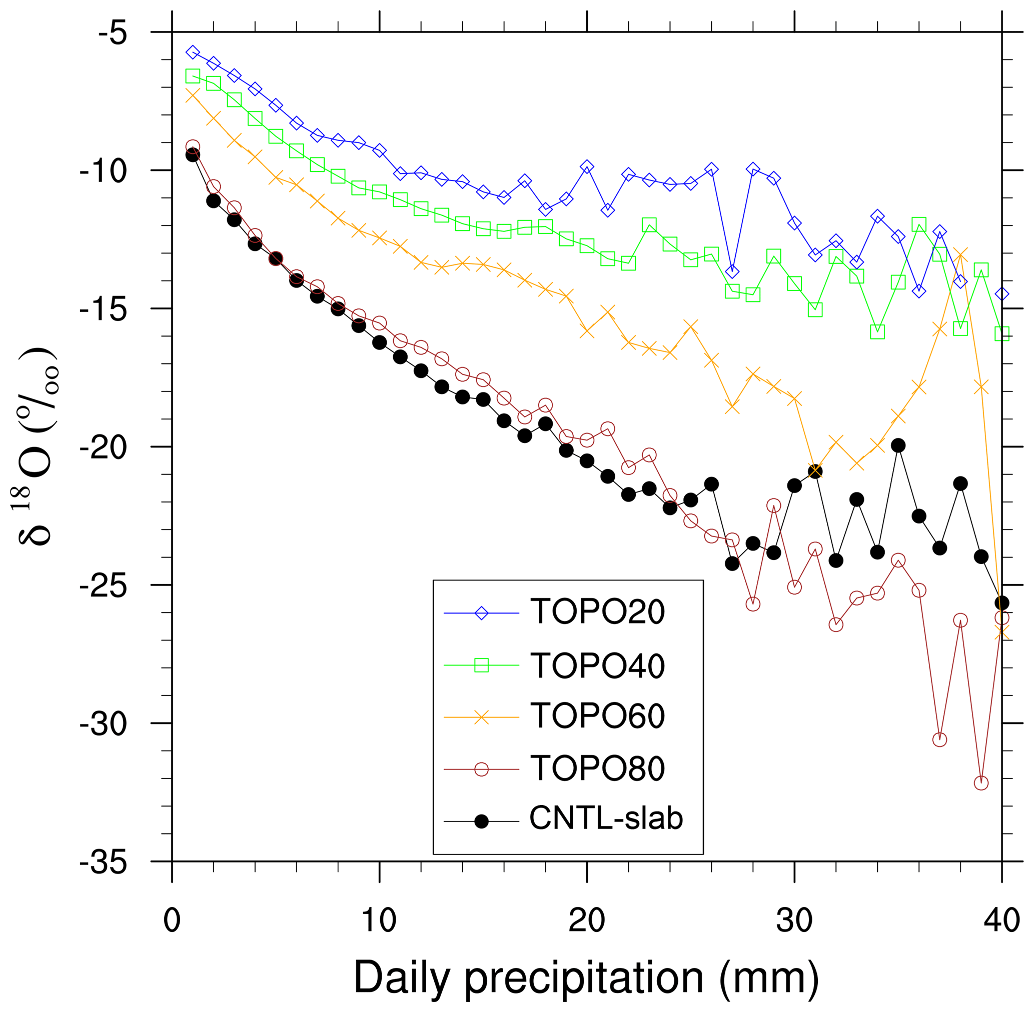
Figure 14 ECHAM δ¹⁸O_p (‰) versus the daily summertime precipitation rate (mm day⁻¹) on the Tibetan Plateau. ECHAM δ¹⁸O_p decreases with increasing precipitation under all elevation scenarios, but is greater in high-elevation scenarios than in low-elevation scenarios.

Sub-cloud reevaporation occurs within an unsaturated air column as falling raindrops undergo kinetic fractionation and become isotopically enriched (Stewart, 1975). Enrichment is reduced in heavier rain where the relative humidity is high, resulting in the observed anticorrelation between δ¹⁸O_p and the precipitation rate referred to as the amount effect. To quantify this enrichment due to sub-cloud reevaporation, we show δ¹⁸O_p against daily precipitation (Fig. 14). The slope of this δ¹⁸O_p–precipitation relationship denotes the strength of the amount effect. In low-elevation scenarios, the δ¹⁸O_p–precipitation slope is shallower (Fig. 14), indicating a weaker amount effect and stronger sub-cloud reevaporation even at high precipitation rates.

This shallow sub-cloud evaporation slope results in the shallower meridional δ¹⁸O_p gradient on the Tibetan Plateau in low-elevation scenarios. In each individual elevation scenario, the enrichment of δ¹⁸O_p due to sub-cloud evaporation is stronger at higher latitudes as there are more instances of lower precipitation rates at higher latitudes than at lower latitudes (Fig. 15). As a result of this different distribution of precipitation, rainfall at higher latitudes is more enriched than that at lower latitudes. To further compare this contribution of sub-cloud reevaporation with surface recycling, the excess enrichment of δ¹⁸O_p due to sub-cloud reevaporation is quantified by the δ¹⁸O_p difference at high and low precipitation rates, weighted by precipitation rates (Table 3). The excess enrichment due to sub-cloud reevaporation is much larger than that due to surface recycling and decreases with reduced elevation.

Figure 15 Relative occurrence (%) of summer daily precipitation rates on the Tibetan Plateau for lower latitudes (averaged over 30–32^∘ N, 85–100^∘ E) and higher latitudes (averaged over 34–36^∘ N, 85–100^∘ E). Only two elevation scenarios (CNTL and TOPO20) are shown here as the other scenarios are identical to these two. Low precipitation rate events are more frequent at higher latitudes than at lower latitudes under all elevation scenarios. See Fig. 13 for a demonstration of how this rainfall distribution impacts δ¹⁸O_p.

To explain this stronger sub-cloud reevaporation in low-elevation scenarios, we refer to the kinetic fractionation process in ECHAM5 during the partial evaporation of raindrops. As shown in Hoffmann et al. (1998), kinetic fractionation in ECHAM5 is formulated as follows:

$$\begin{array}{}\text{(8)}& {\displaystyle }{\displaystyle }\mathit{\alpha }={\displaystyle \frac{\mathrm{RH}}{\frac{D}{\widehat{D}}(\mathrm{RH}-\mathrm{1})+\mathrm{1}}},\end{array}$$

where α is the fractionation factor, $D\times {\widehat{D}}^{-\mathrm{1}}$ represents the ratio of diffusivities between ¹⁶O and ¹⁸O and has the constant value of 0.9727, and RH is the effective relative humidity of the grid box. To estimate how this kinetic fractionation changes between different elevation scenarios, we approximated the effective relative humidity to be the total-column-averaged RH. As seen in Fig. S11, the total-column-averaged RH at any given precipitation rate is higher in high-elevation scenarios than that in low-elevation scenarios. Specifically, when the precipitation rate is very high at 40 mm day⁻¹, the RH is at ∼100 % in the CNTL, suggesting very little kinetic fractionation and weak sub-cloud reevaporation. In comparison, in TOPO20 the RH is much lower at ∼85 %, indicating the presence of sub-cloud reevaporation even at high precipitation rates.

In summary, meridional δ¹⁸O_p gradients on the Tibetan Plateau decrease with lower elevation, and this reduction is due to stronger sub-cloud evaporation in low-elevation scenarios.

4 Discussion

4.1 Processes impacting paleoaltimetry

The use of δ¹⁸O_p as a paleoaltimeter is based on the principle that atmospheric vapor becomes saturated and condenses under forced ascent in orographic regions leading to the preferential rainout of ¹⁸O. Observations of meteoric δ¹⁸O in orographic regions support the use of stable isotope paleoaltimetry and show a robust and significant decreasing relationship in δ¹⁸O_p with surface elevation (e.g., Poage and Chamberlain, 2001; Fiorella et al., 2015; Li and Garzione, 2017) that can be modeled by Rayleigh distillation (Rowley and Garzione, 2007). However, there is no a priori reason that modern δ¹⁸O–elevation relationships should hold in the past when surface elevations and associated atmospheric conditions were different (e.g., Ehlers and Poulsen, 2009; Poulsen et al., 2010; Feng et al., 2013; Botsyun et al., 2016).

Our ECHAM5 results confirm that the processes that govern δ¹⁸O_p vary spatially and change in response to changes in surface elevation (Fig. 17). Across the Himalayan front, δ¹⁸O_p generally decreases with elevation, particularly in scenarios with high Himalayan elevations. However, Rayleigh distillation often does a poor job of explaining the δ¹⁸O_p–elevation relationship in the Himalayan–Tibetan region. There are two primary reasons. Firstly, local processes including convection and surface recycling can dominate the land surface exchange of vapor (Fig. 10). These local processes are especially strong under low-elevation scenarios in monsoonal regions, where forced ascent is weak, and in the western Himalayas. Secondly, in regions with multiple moisture sources, the mixing of air masses with different δ¹⁸O can cause the δ¹⁸O_p–elevation signal to deviate from that expected from Rayleigh distillation. The transitional region in the Himalayas, which receives moisture from both the Arabian Sea and the Bay of Bengal, is such a case (Fig. S7). On the Tibetan Plateau, the meridional δ¹⁸O_p gradient decreases in response to reduced elevation. This meridional δ¹⁸O_p gradient is primarily controlled by sub-cloud reevaporation under modern elevations. Sub-cloud reevaporation increases due to wetter conditions in low-elevation scenarios, reducing the meridional δ¹⁸O_p gradient. Our conclusions are similar to those of Feng et al. (2013) for the North American Cordillera, in which it was shown that the isotopic fractionation of precipitation was not primarily due to Rayleigh distillation.

Our results also highlight the large influence that the choice of moisture source characteristics has on RDM δ¹⁸O_p and are consistent with those of Botsyun et al. (2016). When we use fixed T and RH, ECHAM5 and RDM δ¹⁸O_p agreement is poor with considerable enrichment in RDM. When we use ECHAM5 T and RH, the agreement is considerably improved. This change in moisture sources represents elevation-induced climate change unrelated to rainout and not captured by Rayleigh distillation. The overall impact from T and RH (red diamonds in Figs. 8, 9) is a slight underestimation in high-elevation scenarios and a severe overestimation in low-elevation scenarios (e.g., by ∼100 % in TOPO20 in the IM region).

4.2 Implications for δ¹⁸O_p paleoaltimetry

As discussed above, δ¹⁸O_p paleoaltimetry is only appropriate for monsoonal regions in high-elevation scenarios. Nonetheless, proxy δ¹⁸O_p from sites across the Himalayan–Tibetan region have been used to infer paleoaltimetry throughout the Cenozoic (Fig. 16, Table S1 in the Supplement). We classify these sites into five types indicating their utility for δ¹⁸O_p paleoaltimetry.

Figure 16 Map of δ¹⁸O_p paleoaltimetry sites (filled circles) plotted on surface elevation (shaded). Sites are classified by their type (see Sect. 4.2 for more details on the categories and Table S1 for a list of the sites).

As shown in Fig. 16 (black dots), the modern δ¹⁸O_p–elevation relationship is well captured by ECHAM5 and well represented by the Rayleigh distillation process under high-elevation scenarios for 7 of 50 sites located on the high Himalayas. However, for these seven sites, the δ¹⁸O_p–elevation relationship breaks down as the height of the Himalayan–Tibetan orogen is reduced. For 13 of 50 sites in central Tibet (green dots), there is no direct δ¹⁸O_p–elevation relationship, as elevation is largely uniform and δ¹⁸O_p increases linearly with latitude due to sub-cloud reevaporation and recycling (as outlined in Sect. 3.7). Although it has been proposed that δ¹⁸O_p paleoaltimetry is still possible after removing this meridional δ¹⁸O_p gradient from δ¹⁸O_p (Bershaw et al., 2012), the meridional gradient varies by as much as 70 % with elevation and is largely unknown in the past (as shown in Sect. 3.7); thus, δ¹⁸O_p paleoaltimetry is not appropriate for these sites. For 7 of 50 sites (red dots), elevations are too low, meaning that δ¹⁸O_p has no relationship with elevation and changes very little throughout different elevation scenarios (Fig. 4). As a result, δ¹⁸O_p is not indicative of elevation. For sites in the western and transitional regions (6 of 50), δ¹⁸O_p either relates very little to elevation or exhibits a large range at the same elevation (Fig. S6); thus, it is not appropriate for δ¹⁸O_p paleoaltimetry. Lastly, at sites in northern Tibet (yellow dots, 15 of 50), moisture is mostly diverted by the Tibetan Plateau, Rayleigh distillation is not triggered, and δ¹⁸O_p does not vary with elevation (Fig. 4).

Figure 17 A sketch showing dominant sources/sinks of ¹⁸O in the Himalayas and dominant process impacting δ¹⁸O_p on the Tibetan Plateau for high- and low-elevation scenarios.

Although the δ¹⁸O_p–elevation relationship at sites in monsoonal regions (Fig. 16, black dots) are well explained by Rayleigh distillation in our experiments, δ¹⁸O_p paleoaltimetry should still be applied with care for these sites even under high-elevation conditions due to the influence of climate change. Proxy δ¹⁸O_p values as low as −18 ‰to −16 ‰ are reported for the early Eocene (Ding et al., 2014) and around −14 ‰ for the late Eocene (Rowley and Currie, 2006). These values almost certainly reflect high elevations. Nonetheless, elevation-independent factors, including atmospheric pCO₂ (Poulsen and Jeffrey, 2011) and paleogeography (Roe et al., 2016), add substantial uncertainty to the quantification of past surface elevations.

4.3 Caveats

Like all models, ECHAM has limitations. Most pertinent to this study, ECHAM simulates higher precipitation along the steepest slope of a large mountain than indicated by satellite observations (Roe et al., 2016 and references therein), which is a common problem in most GCMs. The model tends to overestimate the modern precipitation amount and RH on the western Tibetan Plateau. This overestimation also exist in an earlier version of ECHAM (Roe et al., 2016) and in LMDZ-iso (Zhang and Li, 2016). The overestimation of total-column-averaged RH might weaken the sub-cloud reevaporation process on the western plateau, and this weaker reevaporation could potentially lower the meridional δ¹⁸O_p gradient in this region. Another limitation of the model is that sub-grid scale lakes are not included. Although it has been proposed that the lakes provide δ¹⁸O-enriched vapor to the air (Bershaw et al., 2012), under equilibrium conditions the net δ¹⁸O flux to the air should be zero. Despite these limitations, ECHAM's simulation of δ¹⁸O_p compares favorably with natural water isotopic measurements (Li et al., 2016).

Another limitation of our modeling strategy is our use of a slab ocean model, which does not account for ocean circulation changes that would result from the changes in topography that we prescribe. To the best of our knowledge, no existing study has specifically investigated the response to a reduction in the elevations of the Himalayas and the Tibetan Plateau. It is not hard to imagine regional sea surface changes that might influence inland precipitation. For example, we speculate that under lower elevations and weaker monsoon winds, ocean upwelling along the western coast of the Bay of Bengal and the Arabian Sea would be reduced, leading to higher sea-surface temperatures (SSTs). In a study of the East Asian response to historical SST warming, higher SSTs led to greater precipitation over the Indian and Pacific oceans due to enhanced local convection and less precipitation along the Himalayan front, and further weakening of the Asian monsoon (Li et al., 2010). As this example highlights, future studies should incorporate dynamic ocean changes. An associated shortcoming is our prescription of fixed, mean-annual sea-surface δ¹⁸O. To quantify this impact of the seasonal variations of seawater δ¹⁸O on water vapor δ¹⁸O, we estimated the seasonal change of water vapor δ¹⁸O over the ocean using the Craig–Gordon model. Assuming a seasonal variation of 2.5 ‰ in sea water δ¹⁸O (Breitenbach et al., 2010) and monthly SST, RH, and air temperature from our ECHAM5 CNTL case, we estimate that the seasonal change of water vapor δ¹⁸O is within 0.3 ‰. This example illustrates the generally very small influence of seawater δ¹⁸O variations on vapor and precipitation δ¹⁸O.

In this study, we use a series of idealized simulations to investigate the response of water isotopes to mountain uplift and to understand the mechanisms that control δ¹⁸O_p variations in the Himalayas and on the Tibetan Plateau. We do not compare or evaluate our model results directly against proxies, as the simulations are not meant to represent specific time slices in the geologic past, and do not include changes in time-specific boundary conditions such as greenhouse gas composition, vegetation, orbital parameters (Tabor et al., 2018), glacial boundary conditions, tectonic displacement of the Indian subcontinent, or inclusion of the Paratethys. Changes in these boundary conditions, consistent with those that occurred through the Cenozoic, are likely to have a substantial influence on simulated δ¹⁸O_p. For instance, high early Cenozoic atmospheric CO₂ may have increased δ¹⁸O_p over high-elevation regions (Jeffery et al., 2012; Poulsen and Jeffery, 2011) and on the Tibetan Plateau by as much as 8 ‰ (Poulsen and Jeffery, 2011). In addition, Earth's orbital variations have been shown to contribute as much as 7 ‰ to oxygen isotope changes on the Tibetan Plateau (Battisti et al., 2014), which is comparable to the isotope difference from the CNTL to TOPO20 (about −11 ‰) in Fig. 4. These large variations associated with orbital fluctuations are not observed in long records spanning millions of years (Deng and Ding, 2015; Kent-Corson et al., 2009), presumably because the terrestrial proxy archives of δ¹⁸O integrate over orbital time periods.

5 Conclusion

The isotopic composition of ancient meteoric waters archived in terrestrial proxies is often used as a paleoaltimeter under the assumption that rainout during stable air parcel ascent over topography leads to a systemic isotopic depletion via Rayleigh distillation. We use an isotope-enabled GCM, ECHAM5-wiso, to evaluate the extent to which oxygen isotopes can be used as a paleoaltimeter for the Himalayan–Tibetan region and to explore the processes that control the δ¹⁸O–elevation relationship. Overall, our study highlights the myriad processes that influence δ¹⁸O_p in the Himalayan–Tibetan region now and during its uplift.

We find that Rayleigh distillation describes most of the δ¹⁸O_p variation with elevation in the monsoonal regions under high-topography scenarios. In contrast, Rayleigh distillation does a poor job of describing δ¹⁸O_p variation with elevation under high-topography scenarios in the western Himalayas due to the dominance of local convection and surface recycling in the region. When the Himalayan–Tibetan elevations are reduced to below one-half of their modern heights, δ¹⁸O_p exhibits no relationship with elevation. At these reduced elevations, δ¹⁸O fractionation occurs primarily through local convection and surface recycling. On the Tibetan Plateau under modern elevations conditions, δ¹⁸O_p linearly increases with latitude primarily due to sub-cloud reevaporation. The δ¹⁸O_p gradient decreases as the plateau is lowered due primarily to stronger sub-cloud reevaporation under drier conditions and secondarily owing to increased moisture sources from surface recycling. Because of these elevation-independent processes, we conclude that only 7 out of the 50 paleoaltimetry sites are appropriate for δ¹⁸O paleoaltimetry. Taken together, these results indicate that stable isotope paleoaltimetry in the Himalayan–Tibetan region, as in other orogenic regions, is at best a blunt instrument for inferring past surface elevations.