Sediment fluxes dominate glacial–interglacial changes in ocean carbon inventory: results from factorial simulations over the past 780 000 years

Atmospheric CO₂ concentrations varied over ice age cycles due to net exchange fluxes of carbon between land, ocean, marine sediments, lithosphere, and the atmosphere. Marine sediments and polar ice cores archived indirect biogeochemical evidence of these carbon transfers, which resulted from poorly understood responses of the various carbon reservoirs to climate forcing. Modelling studies demonstrated the potential of several physical and biogeochemical processes to impact atmospheric CO₂ under steady-state glacial conditions. However, it remains unclear how much these processes affected carbon cycling during transient changes of repeated glacial cycles and what role the burial and release of sedimentary organic and inorganic carbon and nutrients played. Addressing this knowledge gap, we produced a simulation ensemble with various idealised physical and biogeochemical carbon cycle forcings over the repeated glacial inceptions and terminations of the last 780 kyr with the Bern3D Earth system model of intermediate complexity, which includes dynamic marine sediments. The long simulations demonstrate that initiating transient glacial simulations with an interglacial geologic carbon cycle balance causes isotopic drifts that require several hundreds of thousands of years to overcome. These model drifts need to be considered when designing spin-up strategies for model experiments. Beyond this, our simulation ensemble allows us to gain a process-based understanding of the transient carbon fluxes resulting from the forcings and the associated isotopic shifts that could serve as proxy data. We present results of the simulated Earth system dynamics in the non-equilibrium glacial cycles and a comparison with multiple proxy time series. From this we draw several conclusions. In our simulations, the forcings cause sedimentary perturbations that have large effects on marine and atmospheric carbon storage and carbon isotopes. Dissolved inorganic carbon (DIC) changes differ by a factor of up to 28 between simulations with and without interactive sediments, while CO₂ changes in the atmosphere are up to 4 times larger when interactive sediments are simulated. The relationship between simulated DIC (−1800–1400 GtC) and atmospheric CO₂ change (−170–190 GtC) over the last deglaciation is strongly setup-dependent, highlighting the need for considering multiple carbon reservoirs and multi-proxy analyses to more robustly quantify global carbon cycle changes during glacial cycles.

1 Introduction

During the Quaternary, the Earth's carbon cycle repeatedly shifted between low atmospheric CO₂ during glacial periods and elevated mixing ratios during interglacials in orbitally paced cycles (Petit et al., 1999; Siegenthaler et al., 2005; Lüthi et al., 2008). The reconstructed evolution of atmospheric CO₂ from Antarctic ice cores aligns closely with temperature and is lagged by ice sheet extent, suggesting a close coupling of climate and the carbon cycle (e.g. Shackleton, 2000; Bereiter et al., 2015). However, simulating atmospheric CO₂ changes that are consistent with reconstructed CO₂ and other proxy data is challenging because the observed carbon cycle changes were the result of complex Earth system responses to climate forcing (Schmittner, 2008).

Changing ocean chemistry is often attributed an important role in these cycles because of the considerable size of the marine carbon reservoir (Broecker, 1982a) and because reconstructions show that overall there was likely less carbon stored on land (in vegetation, permafrost, peatlands, and soils) at the Last Glacial Maximum (LGM) than during the current warm period (Yu et al., 2010; Lindgren et al., 2018; Jeltsch-Thömmes et al., 2019). A multitude of physical and biogeochemical processes have been assessed for their contribution to changes in the marine carbon storage on these timescales (e.g. Kohfeld and Ridgwell, 2009; Sigman et al., 2010; Fischer et al., 2010), and their relative importance for the CO₂ difference between the LGM and the late Holocene has been tested in numerical simulations with dynamic ocean models (e.g. Brovkin et al., 2012; Menviel et al., 2012). Changes in ocean circulation and increased CO₂ solubility due to lower temperatures contributed to the lower glacial atmospheric CO₂ concentration (Broecker, 1982a; Smith et al., 1999; Brovkin et al., 2007; Sigman et al., 2010; Fischer et al., 2010), while increased salinity and surface ocean dissolved inorganic carbon (DIC) concentrations due to lowered sea levels tend to counteract this effect by stimulating CO₂ outgassing to the glacial atmosphere (Weiss, 1974; Broecker, 1982a; Brovkin et al., 2007). Furthermore, reduced CO₂ outgassing from the Southern Ocean due to a greater extent of sea ice isolating the surface ocean from the atmosphere and enhanced stratification due to brine rejection during sea ice formation are other physical processes suggested to have affected the glacial carbon cycle (Stephens and Keeling, 2000; Bouttes et al., 2010).

Marine biogeochemical processes that lead to lower atmospheric CO₂ include a shift in organic carbon remineralisation to greater depths and an increased export production due to increased nutrient supply to the whole ocean. These processes have opposite effects on export production. Nutrient input from the weathering of emerged shelves (phosphate), changes in nitrogen fixation and denitrification, and enhanced dust deposition (iron, silica) could have boosted export productivity (Broecker, 1982b; Martin, 1990; Pollock, 1997; Deutsch et al., 2004). On the other hand, a reduced return rate of nutrients from the deep ocean into the surface in response to deeper remineralisation might have resulted in more efficient nutrient utilisation and less export.

In a (hypothetical) closed atmosphere–ocean system, the combination of these processes results in increased marine carbon storage during glacials, but not necessarily in the open Earth system, because the carbon removed from the surface ocean and atmosphere by these processes could have been sequestered as particulate carbon in marine sediments in addition to DIC in the water column. Constraints on glacial atmospheric CO₂ can be reconciled with increased and decreased marine DIC inventory in an open system (Jeltsch-Thömmes et al., 2019; Kemppinen et al., 2019), though reproducing reconstructed carbon isotopic changes in the atmosphere and ocean seems to require elevated DIC at the LGM (Jeltsch-Thömmes et al., 2019).

It is very probable that changing sedimentary carbonate and particulate organic carbon (POC) burial played a relevant role in glacial–interglacial carbon cycle changes by altering seawater carbonate chemistry, carbonate ion concentrations, carbon isotope ratios, and oxygenation. In particular, continental shelves have emerged from the ocean during glacial sea level low stands and provided new reef habitats and carbonate deposition environments during deglaciations and interglacials (e.g. Broecker, 1982b; Opdyke and Walker, 1992; Ridgwell et al., 2003; Brovkin et al., 2007; Menviel and Joos, 2012). Additionally, carbonate burial changes in the open ocean have been regarded as amplifiers of marine carbon uptake (e.g. Archer and Maier-Reimer, 1994; Kohfeld and Ridgwell, 2009; Schneider et al., 2013; Roth et al., 2014; Kerr et al., 2017; Kobayashi et al., 2021). Organic carbon burial is also prone to vary in response to changes in the rain rate of POC sinking to the sea floor and altered oxygenation. Previous model simulations showed that interactive sediments including POC burial greatly affect atmospheric CO₂ and carbon isotope variations through the burial–nutrient feedback, whereby enhanced burial of organic-bound carbon and nutrients reduces export production (Tschumi et al., 2011; Roth et al., 2014; Jeltsch-Thömmes et al., 2019; Jeltsch-Thömmes and Joos, 2023). Reconstructions of marine burial changes over the last glacial cycle suggest a reduction in globally integrated inorganic carbon burial (Cartapanis et al., 2018; Wood et al., 2023) during the last glacial period but increased organic (Cartapanis et al., 2016) sedimentary carbon burial. The magnitudes of both changes are uncertain due to the spatial heterogeneity of sedimentary burial and the inherently local nature of marine archives but possibly of comparable magnitude to terrestrial carbon stock changes (Cartapanis et al., 2016, 2018). These findings demonstrate that organic and inorganic sedimentary changes and imbalances with weathering fluxes need to be considered when quantifying carbon reservoir changes of the ocean, atmosphere, and land and interpreting the reconstructed changes in CO₂, carbonate ion concentrations, isotopes, and nutrients over glacial cycles.

Model-based estimates of carbon and carbon isotope inventory differences between glacial and interglacial periods are complicated by temporal carbon cycle imbalances during the continuously evolving climate of glacial cycles. This is particularly challenging when simulating dynamic elemental cycling in and burial from reactive marine sediments and the input of elements by weathering and volcanic outgassing because of long-lasting re-equilibration and memory effects in carbon and nutrient fluxes and particularly isotopic changes (Tschumi et al., 2011; Jeltsch-Thömmes and Joos, 2020). Dynamic sedimentary adjustment, i.e. the equilibration of sedimentary dissolution and remineralisation to changes in bottom water which slowly diffuse into sedimentary porewater, and imbalances between the supply (weathering) and loss (sedimentary burial) of carbon and nutrients increase the equilibration time of atmospheric CO₂ by a factor of up to 20 to several tens of thousands of years, and the resulting δ¹³C perturbations take hundreds of thousands of years to recover (Roth et al., 2014; Jeltsch-Thömmes et al., 2019; Jeltsch-Thömmes and Joos, 2023). Importantly, the equilibration timescales are longer than typical interglacials in the late Pleistocene, which opens up the possibility for memory effects that span several glacial cycles.

A caveat of several modelling studies attempting to quantify carbon reservoir sizes at the LGM is that they assume a steady-state carbon cycle in a closed (atmosphere–ocean–land, excluding interactive marine sediments) system and do not account for the history of environmental changes that pre-dated the LGM but could have introduced long-lasting memory effects. Transient simulations of an entire glacial cycle with a fully dynamic marine and sedimentary carbon cycle showed that time lags in the carbon cycle response to orbital forcing add constraints for the identification of the processes that caused glacial CO₂ changes (Menviel et al., 2012). In particular, imbalances between marine carbon burial and continental weathering and the long marine residence time of phosphate delay the CO₂ increase during the temperature rise of deglaciations. Accounting for these long-term effects in the experimental design, transient simulations of more than one glacial cycle showed that reconstructed atmospheric CO₂ and benthic marine δ¹³C changes over the last 400 kyr could be reasonably well simulated with a combination of physical (radiative and ocean volume changes) and biogeochemical processes (carbonate chemistry and land carbon changes, temperature-dependent remineralisation depth, additional nutrient supply during glacials, shallow water carbonate burial changes;  Ganopolski and Brovkin, 2017). However, shallow-water carbonate burial was prescribed and POC burial was not included in the simulations, which begs the following question: what were the effects of the considered processes on glacial–interglacial atmospheric CO₂ and carbon isotopic ratios changes if the sediments were dynamically calculated? Recently, simulations of glacial–interglacial cycles beyond the Mid-Brunhes transition (∼ 430 ka) were run with a box model (Köhler and Munhoven, 2020) and a purely physical model (Stein et al., 2020), which were unable to capture transient and spatially heterogeneous interactive sediments. CLIMBER-2, a fully coupled intermediate-complexity Earth system model, was run stepwise over the last 3 Myr, but the results were not analysed for the carbon cycle dynamics (Willeit et al., 2019).

Here we examine systematically how the transient buildup and dissolution of marine sediments on glacial–interglacial timescales affect the carbon cycle changes produced by the various processes suggested to be relevant on these timescales, a gap left by previous studies. We explicitly consider the burial of organic carbon and opal, in addition to CaCO₃. Instead of searching for the most likely scenario that reconciles the vast proxy evidence, we attempt to gain a more complete process understanding and overview of the proxy-relevant signals that these processes cause in the presence of weathering–burial imbalances. With this goal, we extend factorial simulations of multiple simplified physical and biogeochemical forcings in a marine-sediment- and isotope-enabled intermediate-complexity Earth system model over the last 780 kyr and compare the resulting carbon and carbon isotopic signals to reconstructions. The long timescale is chosen to avoid biases resulting from steady-state assumptions and to account for the possibility of memory effects under a continuously varying climate and carbon cycle that could span multiple glacial cycles. Consequently, all carbon stores are achieved dynamically rather than being prescribed. We present two sets of simulations with and without interactive sediments to distinguish the role of interactive sediments in the carbon cycle changes caused by the tested forcings over reoccurring glacial cycles of the last 780 kyr.

2 Methods

2.1 Bern3D v2.0s

We simulated the Earth system's transition through the last 780 kyr of glacial cycles with the intermediate-complexity Earth system model Bern3D v2.0s, which has an irregular 41×40 grid (lowest resolution: lat × long $=\mathrm{5}\mathit{°}\times \mathrm{10}\mathit{°}$ in the North Pacific; highest resolution: lat × long $=\mathrm{3}\mathit{°}\times \mathrm{7}\mathit{°}$ in the equatorial Atlantic) in the horizontal and 32 logarithmically spaced ocean depth layers. The model combines modules for 3D physical ocean dynamics, marine biogeochemistry, marine interactive sediments, and atmospheric energy–moisture balance.

The physical ocean component transports tracers through the ocean by advection, convection, and diffusion. Euphotic zone production depends on temperature, light, sea ice cover, and nutrient (phosphate, iron, silica) availability (Parekh et al., 2008; Tschumi et al., 2011) and explicitly calculates carbon isotope dynamics (Jeltsch-Thömmes et al., 2019). In our setup, a fraction of the particulate organic matter formed in the surface ocean is instantly remineralised following an oxygen-concentration-dependent version of the globally uniform Martin curve (Battaglia and Joos, 2018), and particulate inorganic carbon and opal dissolution occurs according to globally uniform e-folding profiles. The remaining solid particles reaching the sediment–ocean interface enter reactive sediments, where they are preserved, remineralised, or redissolved depending on dynamically calculated porewater chemistry and are mixed by bioturbation (Tschumi et al., 2011). CaCO₃ dissolution rates in the sediments are determined from the porewater saturation state, and POC remineralisation is parameterised by a linear dependence on porewater O₂ (Heinze et al., 1999; Tschumi et al., 2011). The model contains 10 layers of reactive sediments. As matter gets pushed downward out of the bottom layer (“sedimentary burial”), it is lost to the modelled inventories. These loss fluxes of C, ¹³C, Alk, P, and Si are at equilibrium compensated for by a corresponding solute input flux from land into the coastal surface ocean. The (pre-industrial, PI) land–sea mask and bathymetry are fixed throughout the spin-up and simulations.

2.2 Model spin-up with interglacial boundary conditions

We spun up the model with pre-industrial boundary conditions in three stages, sequentially coupling all modules, for computational efficiency. Firstly, we forced the ocean circulation and then the atmosphere–ocean carbon cycle as a closed system with pre-industrial climatic conditions and prescribed CO₂ for 20 kyr. In the next step, the sediment module is coupled and terrestrial solute supply (phosphate, alkalinity, DIC, DI¹³C, and Si) to the ocean is set to dynamically balance the loss through sedimentary burial for 50 kyr. At the end of this stage, the solute input flux, hereafter named “weathering input”, required to balance sedimentary burial is diagnosed (Table S1 in the Supplement) and kept constant for the rest of the spin-up procedure and throughout our transient experiments. Until this stage, atmospheric CO₂ and δ¹³C were prescribed. The spun-up model for the pre-industrial was then run for 2000 years as an open system (freely evolving CO₂ and δ¹³C) with radiative forcing that varied linearly from the PI to the slightly different MIS19 conditions, the starting point of our experiments. The total length of the spin-up to this point was 72 kyr. To avoid large drifts in carbon isotopes and alkalinity (Jeltsch-Thömmes and Joos, 2023; explained at the end of Sect. 3.5) in the simulations with the forcings that perturbed the carbon cycle the most (PO4, REMI, LAND, CO2T, BGC, ALL; described in the next section), we ran the fully interactive model with each respective forcing for two glacial cycles (215 kyr) before starting our experiments. We discuss the relevance of initial conditions and imbalances of the geologic carbon cycle at the end of the article. Model limitations due to constant terrestrial solute supply are discussed in the Supplement (Sect. S2).

2.3 Experimental design

Data constraints on carbon cycle forcings are too sparse to know exact magnitudes and timings of the forcings that might have varied spatially and temporarily over the last eight glacial cycles. An inverse estimation of the forcings from the resulting proxy signals requires a different simulation ensemble and is beyond the scope of our study. Rather than trying to guess the most proxy-consistent forcing amplitudes and patterns, we designed seven simplified forcings, each with one exemplary magnitude, to simulate the generic effects of processes that have been identified as glacial–interglacial carbon cycle drivers. Except for the orbital changes, which were calculated following Berger (1978), Berger and Loutre (1991), and the reconstructed CO₂, N₂O, and CH₄ curves (Loulergue et al., 2008; Joos and Spahni, 2008; Bereiter et al., 2015; Etminan et al., 2016), which we used to calculate the radiative forcing of greenhouse gas changes, the amplitudes of the forcings were set to cause noticeable CO₂ or circulation shifts, informed by previous studies (e.g. Tschumi et al., 2011; Menviel and Joos, 2012; Menviel et al., 2012; Jeltsch-Thömmes et al., 2019; Pöppelmeier et al., 2021). We produced time series of these forcings by defining a maximum forcing amplitude for the LGM and a minimum for the Holocene and then modulating this amplitude by reconstructed relative changes in the temporal evolution of either Antarctic ice core δD (Jouzel et al., 2007) or benthic δ¹⁸O (Lisiecki and Raymo, 2005) for each year (Fig. 1). The choice of the isotope record for calculating the instantaneous forcing depends on whether we expect the forcing to evolve synchronously with temperature like δD or have a time lag similar to δ¹⁸O (see Sect. S2 for a discussion of the limitations). In all simulations, we prescribed the radiative effect of CO₂ in the atmosphere so that all simulations have the same radiative forcing from greenhouse gases despite differences in simulated CO₂.

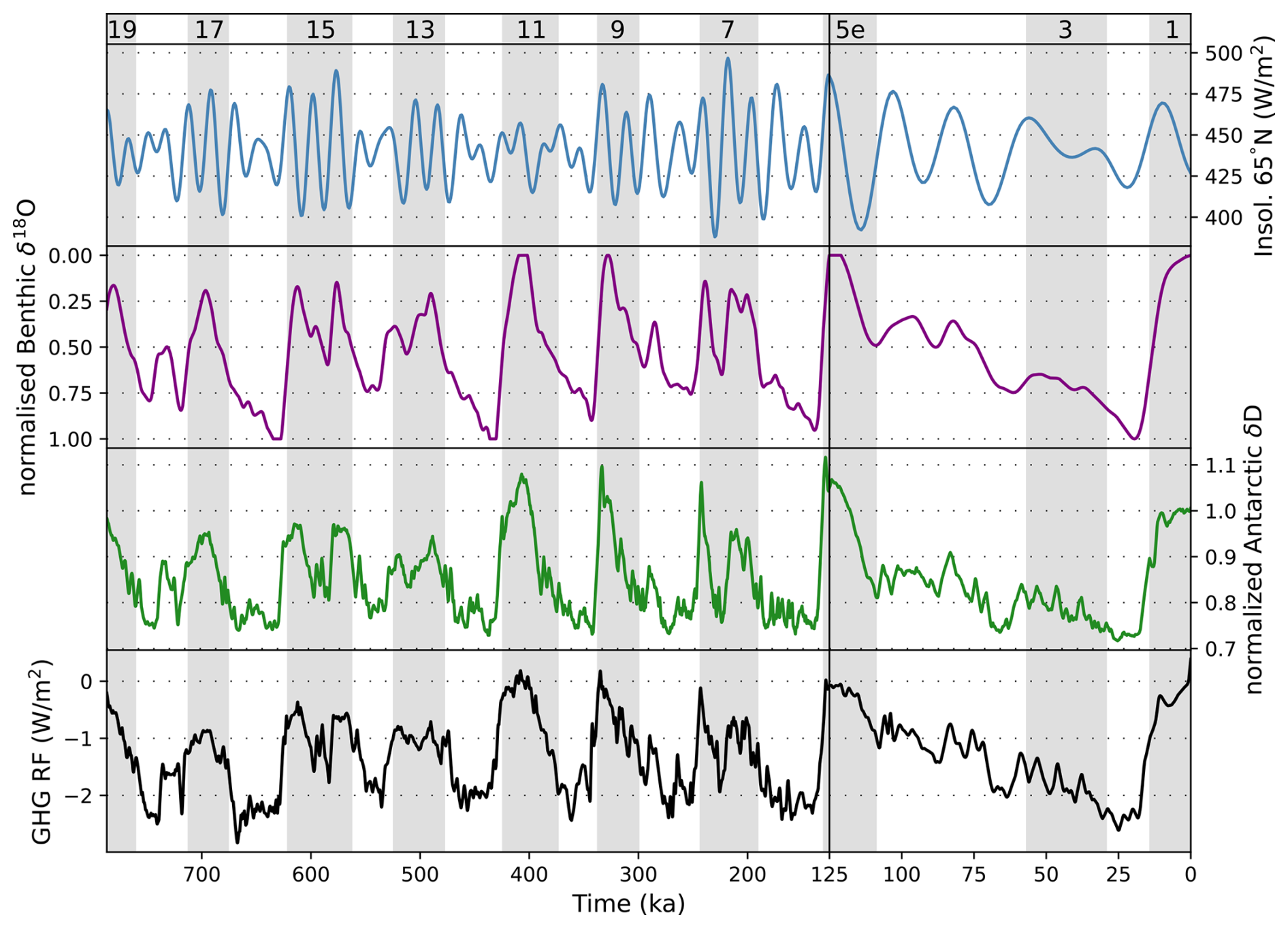
Figure 1 Forcing time series. Insolation changes (top panel) are calculated according to Berger (1978) and Berger and Loutre (1991). The δ¹⁸O forcing (second panel) is the LR04 stack (Lisiecki and Raymo, 2005), smoothed by averaging over a 10 000-year moving window and normalised to the LGM–PI difference. The δD forcing (third panel) is taken from Jouzel et al. (2007) and normalised to the LGM–PI difference. The radiative forcing (RF) of CO₂, N₂O, and CH₄ (greenhouse gases, abbreviated to “GHG” in the bottom panel) is calculated from Bereiter et al. (2015), Loulergue et al. (2008), and Joos and Spahni (2008) following Etminan et al. (2016). The grey shading indicates uneven marine isotope stages (MISs).

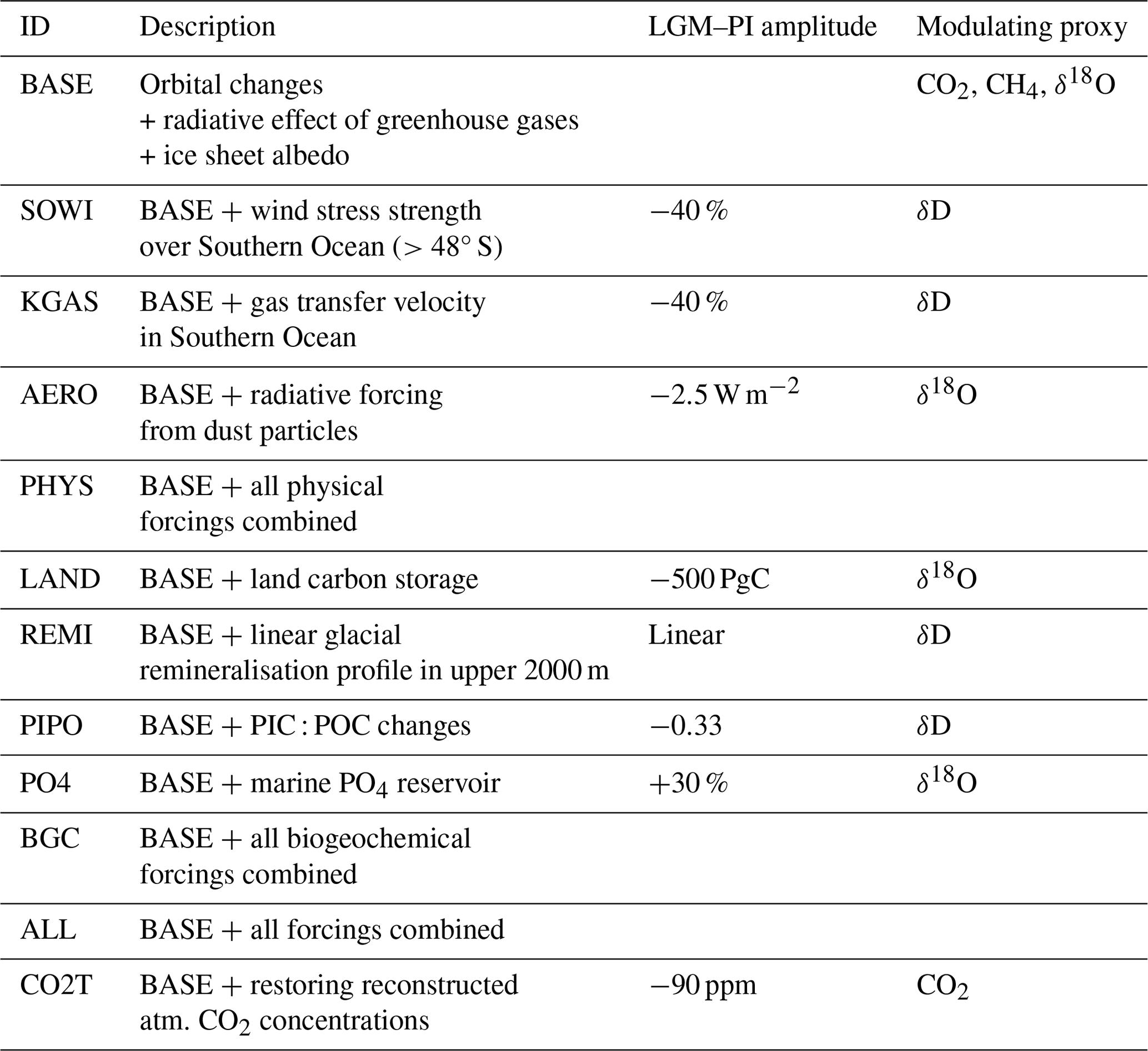
Specifically, we performed one “base” run with orbital and radiative forcing only and one model run for different forcings, each added to the base forcing, and combinations of the individual forcings to study non-linear effects that appear when processes interact. All of these experiments are run once with and once without interactive sediments, to examine the effect of sediment perturbations on the results. The forcings and their rationales are described below. The experiments are summarised in Table 1.

The application of the standard forcing in the simulation BASE causes temperature changes associated with orbital, albedo, and greenhouse gas changes which affect solubility, sea ice, and circulation, e.g. slightly weakening AMOC (by up to 4.5 Sv; Fig. S8 in the Supplement), and resulting in younger deep-water masses in the Atlantic and Pacific during the LGM than at the PI, which is inconsistent with proxy data and thus indicates that additional Earth system changes must have occurred (Pöppelmeier et al., 2021). To achieve an older glacial deep ocean (diagnosed with an ideal age tracer), we reduced the wind stress south of 48° S by a maximum of 40 % (simulation SOWI) temporally changing proportionately to the δD change because we assume that wind strength over the Southern Ocean evolved without temporal lags to Antarctic temperature. As a result, the South Pacific downwelling is strengthened by up to 1.5 Sv locally in glacials, AMOC strength is further reduced by up to 1 Sv, and the simulated deep-ocean age is ∼ 100 years older in the LGM than in the PI, close to published model estimates (Schmittner, 2003). In this setup, changing wind stress only affects the circulation, not the piston velocity of gas exchange, which is forced by a wind speed climatology. For an independent assessment of the effect of wind speed changes on sea–air gas exchange, we performed a simulation in which we decreased the piston velocity in the Southern Ocean by a maximum of 40 % (KGAS), also following the evolution of δD. Next, we simulated the additional negative radiative forcing due to increased aerosol loads in the glacial atmosphere (AERO; e.g. Claquin et al., 2003) by further reducing the total radiative forcing by a maximum of 2.5 W m⁻² during the LGM, modulated by the δ¹⁸O record based on the reconstructed correlation between dust and δ¹⁸O (Winckler et al., 2008; similar to the study of long-term circulation changes in Adloff et al., 2024a). Under this forcing, the AMOC does not shut down but weakens by up to 12 Sv relative to the PI during glacial maxima due to density changes and sea ice advance in the North Atlantic (the model behaviour under this forcing is described more extensively in Adloff et al., 2024a), and deep North Atlantic water mass age rises to up to 1000 years.

In terms of biogeochemical forcings, we mimicked five processes that would have occurred during glacial cycles but are not dynamically simulated by our model. Firstly, we added a terrestrial carbon sink/source by removing/adding 500 PgC during deglaciation/ice age inception to simulate the marine impact of climate-driven carbon cycle changes on land (LAND; Jeltsch-Thömmes et al., 2019). Secondly, we reduced nutrient limitation on glacial export production (PO4) with a globally uniform addition of phosphate, the only export-limiting nutrient in our model setup, into the surface ocean, increasing the marine phosphate inventory by 30 % during the glacial maxima. The time series of LAND and PO4 are proportional to δ¹⁸O changes because we assume that both are lagging behind temperature changes due to continental ice sheets and changing terrestrial environments. Effectively, our nutrient forcing reduces nutrient limitation globally. Rather than simulating the effects of different nutrient inputs in different regions (e.g. iron in the Southern Ocean, phosphate at shelves), we decided to group all these in one simulation with a global forcing because their net effect, increased export production, would be the same in our model, just in different regions. This is the only forcing that we did not apply to the model without interactive sediments because, while nutrients can be added to the surface ocean periodically, there is no simple way of artificially extracting nutrients from the ocean in return. Thirdly, we reduced the speed of aerobic organic matter remineralisation in the ocean to simulate temperature-driven changes in respiration rates by transitioning between the standard, pre-industrial Bern3D particle profile (Martin scaling) during interglacials and a linear profile in the first 2000 m of the water column (REMI; Fig. S9), following the δD record, since we assume that remineralisation changes happened synchronously with temperature change. Fourthly, we reduced the PIC : POC rain ratio by 33 % in the LGM (PIPO) and similarly modulated the forcing time series with the δD record. This simulation mimics the effect of an ecological shift in marine primary producers on the composition of biogenic marine particles. Fifthly, we performed one run in which we let the model dynamically apply external alkalinity (ALK) fluxes (in addition to the constant terrestrial solute supply applied in each simulation; see spin-up methodology) to restore the reconstructed atmospheric CO₂ curve (CO2T). In this simulation, the model evaluates the difference between the simulated and reconstructed CO₂ at each time step and adds or removes the marine ALK required to cause the necessary compensatory air–sea carbon flux from the surface ocean. ALK changes, e.g. due to changes in shallow carbonate deposition or terrestrial weathering, are an effective lever for atmospheric CO₂ change (e.g. Brovkin et al., 2007), and this additional run shows the long-term changes in marine biochemistry if this was the dominant driver of glacial–interglacial atmospheric CO₂ change.

Table 1 Forcing scenarios. Simulations are run in two configurations: the standard setup with interactive sediments and a closed-system setup without sediments (except PO4).

For the discussion of the simulations, we quantify the factorial effect of the simulated forcings on different carbon cycle metrics. In simulation BASE, only the standard forcing is active (see Table 1); hence the factorial effect of the standard forcing is equal to the simulated change:

$$\mathrm{fBASE}=\text{BASE}.$$

In the simulations that combine the standard forcing with one other forcing, the factorial effect of the additional forcing is the difference between the respective simulation and BASE:

$$\mathrm{fFORC}=\text{FORC}-\mathrm{fBASE}.$$

In simulations PHYS, BGC, and ALL, several forcings are combined. We use these simulations to determine non-linearities by calculating the difference between the results of these simulations and the linear addition of the individual effects of the active forcings:

$$\begin{array}{c}{\displaystyle }\mathrm{nlPHYS}=\text{PHYS}-(\mathrm{fBASE}+\mathrm{fKGAS}+\mathrm{fSOWI}+\mathrm{fAERO})\\ {\displaystyle }\begin{array}{rl}\mathrm{nlBGC}& =\text{BGC}-(\mathrm{fBASE}+\mathrm{fREMI}+\mathrm{fPO}\mathrm{4}+\mathrm{fPIPO}\\ & +\mathrm{fLAND})\end{array}\\ {\displaystyle }\mathrm{nlADD}=\text{ALL}-\text{PHYS}-\text{BGC}+\text{BASE}\\ {\displaystyle }\mathrm{nlTOT}=\mathrm{nlPHY}+\mathrm{nlBGC}+\mathrm{nlADD}.\end{array}$$

3 Results

The general response of marine biogeochemistry to the applied forcings has been tested and described in previous studies (e.g. Tschumi et al., 2008, 2011; Menviel and Joos, 2012; Menviel et al., 2012; Jeltsch-Thömmes et al., 2019; Jeltsch-Thömmes and Joos, 2020); therefore, we just provide a brief summary here and focus more extensively on their effect on the sediment fluxes. A more detailed analysis of the model behaviour under each forcing is provided in the Supplement.

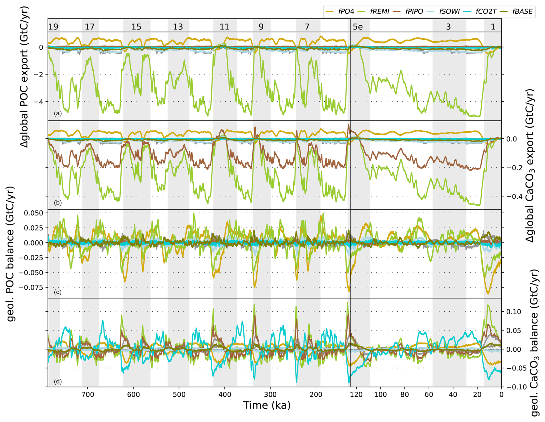
Figure 2 Transient changes in POC and CaCO₃ export production and geologic imbalance (i.e. the difference between accumulation of these materials in marine sediments and the lithosphere minus the constant supply into the surface ocean that mimics terrestrial weathering and volcanism in our simulations) due to the applied forcings. Shown are the factorial differences from the pre-industrial for each simulation. The results that are explicitly mentioned in the text are shown in colour, and the others are shown in grey. Grey shading indicates uneven MIS as indicated at the top of the figure. See Fig. S10 for absolute rather than factorial differences from the pre-industrial in each simulation.

In our setup, carbon exchange between the atmosphere, ocean, and sediments and the burial flux to the lithosphere reacts to climatic and biogeochemical changes, while weathering input fluxes of DIC, ALK, PO${}_{\mathrm{4}}^{\mathrm{3}-}$, Si, and ¹³C are constant over time. Thus, a carbon flux imbalance arises in our simulations in response to the applied forcings (Fig. 2 for factorial differences and Fig. S10 for absolute differences). All forcings except fPO4 reduce global export production during glacial phases (Fig. 2a and b), either due to cooling and expanding sea ice or increased nutrient limitation. In addition to export production, the net exchange of carbon and other elements between sediments and the ocean is changed by the applied forcings via changing benthic seawater composition, either through circulation, solubility, or biogeochemical changes. Cooling (in fBASE) reduces global sediment accumulation rates of CaCO₃ and POC during glacial phases due to the reduced export production (Fig. 2c and d). In consequence, sequestration of CaCO₃ and POC from the reactive sediments (i.e. sedimentary burial) is also reduced in response to these forcings, since it is governed by the sedimentary mass accumulation rate. Instead, reduced nutrient limitation during glacial phases (fPO4) causes more, rather than less, export production during glacial phases. Deepening of the main remineralisation depth (fREMI) increases the preservation of sedimentary POC during glacials by reducing marine O₂. Hence, under this forcing, POC accumulation is higher during glacial than interglacial phases, while the opposite temporal change occurs for CaCO₃ accumulation due to reduced CaCO₃ export production. Increased ALK supply in simulation CO2T causes larger sedimentary CaCO₃ accumulation during glacial phases when ALK input increases CaCO₃ stability and dissolution events during deglaciations when ALK is removed.

How do the simulated sedimentary changes in our factorial setup compare in magnitude and sign with carbon cycle proxy records?

We discuss this question firstly by focusing directly on changes in the carbon stored as sedimentary organic and inorganic matter and changes in the benthic carbonate system, before studying their effects on four essential carbon cycle metrics: deep-ocean CO${}_{\mathrm{3}}^{\mathrm{2}-}$, atmospheric CO₂, marine DIC, and δ¹³C. Individual proxy records were selected for their resolution or length. This is not an attempt at a comprehensive compilation of proxy records or an attempt to understand individual records in detail. Our simulations are designed to constrain the potential and plausibility of major contributions of the tested forcings to the observed glacial–interglacial atmospheric CO₂ changes, rather than reproducing a full, realistic scenario. We therefore do not expect that any single simulation presented in our study captures all features of the reconstructed carbon cycle changes over glacial–interglacial cycles. Instead, we investigate in isolation the forcings that would have to some extent occurred simultaneously in reality and quantify their effects during eight consecutive glacial cycles. Comparing our results to selected proxy records, we discuss processes behind specific patterns of carbon cycle change and the role of weathering–burial imbalances in these.

3.1 Sedimentary burial and CO${}_{\mathrm{3}}^{\mathrm{2}-}$ concentrations

Reconstructions of global POC burial flux changes over the last glacial cycle (Cartapanis et al., 2016) indicate that POC burial was smallest during interglacials and gradually rose during glacial phases until it peaked during the LGM. fSOWI, fREMI, and fPO4 are the only effects which produce higher POC burial fluxes during glacial maxima than during interglacials (Fig. 2), and the latter two are the only ones strong enough to overprint the opposite effect due to cooling (fBASE; Fig. S10). However, the simulated increase in POC burial already occurs during the glacial inception, such that the highest burial rates persist throughout most of the glacial phase, while, in the reconstructions, they remain close to the interglacial value through MIS4. Reconstructions of global CaCO₃ burial changes over the last glacial cycle (Cartapanis et al., 2018) show that burial rates decreased in most ocean basins during glacial inception but increased in the Southern Ocean, resulting in almost no changes in the global average before MIS3. Physical forcings (e.g. fSOWI in Fig. 2) do not affect global CaCO₃ burial rates during glacial inception, consistent with the reconstruction, while fPO4 and fCO2T produce global burial increases and fPIPO and fREMI produce decreases between MIS5 and MIS3. However, the physical forcings fail to produce lower CaCO₃ burial rates during MIS3 and MIS2. fREMI and fPIPO decrease CaCO₃ burial during MIS3 and MIS2 but cause much larger burial events in MIS1 than reconstructed (Fig. 2; see also Figs. S2–S7).

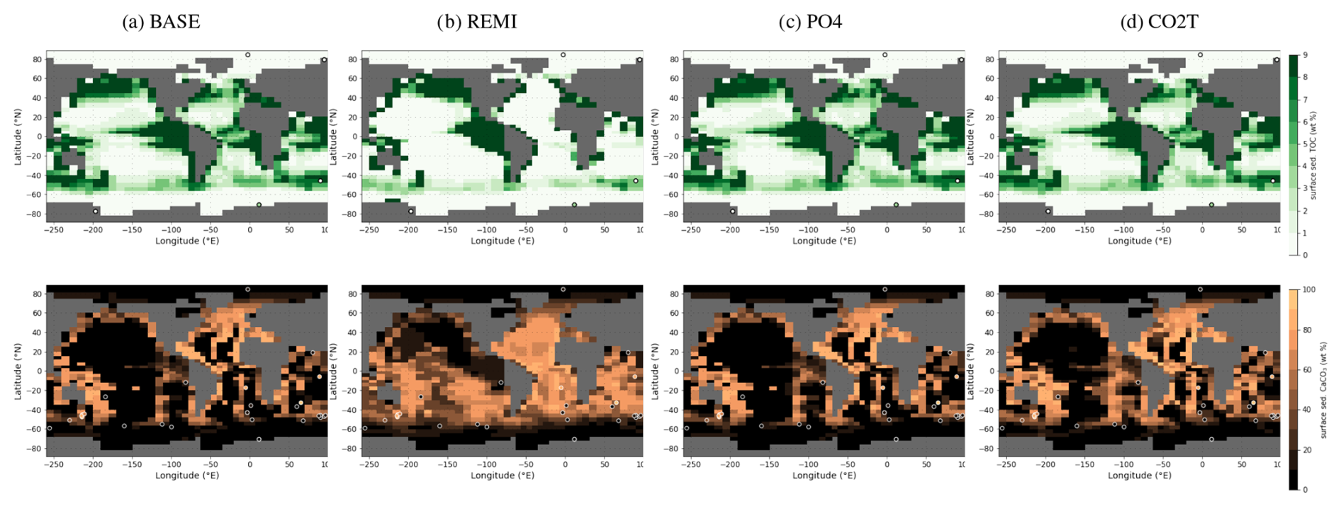
Figure 3 Sedimentary POC and CaCO₃ fractions during the LGM as reconstructed (circles; records for POC and CaCO₃ are from Cartapanis et al., 2016, and Wood et al., 2023, respectively) and in simulations PHYS, REMI, PO4, and CO2T (underlying maps). Shown are only data points that fall into the local benthic grid box of the model. The root-mean-square errors of simulated and reconstructed values are (from left to right) 7.4 wt %, 3.3 wt %, 7.4 wt %, and 6.4 wt % for POC (top row) and 33.6 wt %, 31.5 wt %, 33.3 wt %, and 34.4 wt % for CaCO₃ (bottom row).

Most forcings increase the POC content of surface sediments (top 10 cm) during the LGM (Fig. 3 top row), the exception being fREMI, which decreases POC outside the East Pacific. However, too few reconstructions exist for depths that are consistent with our model bathymetry for a quantitative model–data comparison. For CaCO₃, a few more data points fall within our benthic ocean grid cells. The cooling-related changes (fBASE) included in all simulations reproduce a data-consistent carbonate compensation depth (CCD) in most of the Southern Hemisphere extra-tropics but a CCD that is too high in the tropical South Atlantic and the Indian Ocean and a CCD that is too low off Peru (Fig. 3 bottom row). REMI better captures these tropical CCD changes but produces an extra-tropical CCD that is too low. These model–data differences indicate that different processes might explain the LGM sedimentary composition in different basins, which is not captured by our globally uniform forcings.

The model has been tuned to the pre-industrial CaCO₃ distribution. However, in our study, late Holocene CaCO₃ contents are the result of almost 800 kyr of transient simulation, which results in imbalances in the geologic carbon cycle at the simulation end even though the forcing is that of the Holocene (Table S2). Differences between the dynamically achieved and observed pre-industrial sedimentary composition add context to the size of the simulated sedimentary fluxes and memory effects. The dynamically evolved sedimentary POC content is similar across all simulations, while the CaCO₃ content exhibits large-scale differences (Figs. S11, S12). Simulations with small sediment perturbations during the glacial cycle (e.g. SOWI, AERO, and LAND; Fig. S12) result in CaCO₃ contents that are similar to Holocene estimates. In simulations REMI and PIPO, the large deglacial CaCO₃ burial event results in higher sedimentary CaCO₃ contents in the late Holocene than measured. Simulation CO2T, on the other hand, has less sedimentary CaCO₃ content during the late Holocene than measured. This is the result of strong dissolution due to forced ALK removal from the open ocean during deglaciations, mimicking, for example, coral reef building. It is therefore less likely that sedimentary CaCO₃ was perturbed to the extent simulated in REMI, PIPO, and CO2T.

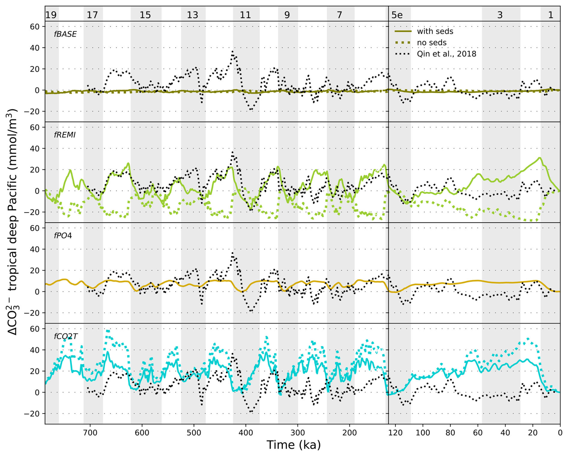
Figure 4 Evolution of CO${}_{\mathrm{3}}^{\mathrm{2}-}$ in the tropical deep Pacific as simulated for fBASE, fREMI, fPO4, and fCO2T (from top to bottom) and reconstructed by Qin et al. (2018). The results of the other forcings are shown in Fig. S13.

Next, we address [CO${}_{\mathrm{3}}^{\mathrm{2}-}$] changes. Kerr et al. (2017) found a repeated pattern of low benthic [CO${}_{\mathrm{3}}^{\mathrm{2}-}$] in the tropical Pacific and Indian oceans during interglacials and high [CO${}_{\mathrm{3}}^{\mathrm{2}-}$] during glacials (difference of 20–55 mmol m⁻³) throughout the last 500 kyr. Qin et al. (2018) found that the same pattern extended over the last 700 kyr, to our knowledge the longest [CO${}_{\mathrm{3}}^{\mathrm{2}-}$] record. Physical forcings (fBASE, fKGAS, fSOWI, fAERO, fPHYS) and fPO4 have little effect on the deep Pacific [CO${}_{\mathrm{3}}^{\mathrm{2}-}$] over glacial cycles (Fig. 4, S13). Under the biogeochemical forcings (fREMI, fPO4, fPIPO, fLAND), the simulated glacial–interglacial [CO${}_{\mathrm{3}}^{\mathrm{2}-}$] difference ranges from a few millimoles per cubic metre (mmol m⁻³) to 50 mmol m⁻³ and is caused by the invasion of CO₂ into the ocean, ALK redistributions within the ocean, and weathering–burial imbalances due to changes in the carbonate export flux and carbonate compensation (Broecker and Peng, 1987; Figs. 4 and S13). fREMI and fCO2T cause the largest [CO${}_{\mathrm{3}}^{\mathrm{2}-}$] changes in the deep equatorial Pacific. For the last glacial cycle, these simulated changes are larger than those reconstructed, suggesting that the forcings cause overly large ALK redistributions within the ocean or carbonate compensation during the last glacial cycle. Interestingly, however, during MIS13–MIS11 and the Mid-Brunhes transition, reconstructed [CO${}_{\mathrm{3}}^{\mathrm{2}-}$] changes in the deep equatorial Pacific were larger than during the last glacial cycle (Qin et al., 2018; Fig. 4). fCO2T and fREMI, which produced larger [CO${}_{\mathrm{3}}^{\mathrm{2}-}$] changes over the last glacial cycle than those reconstructed, produced [CO${}_{\mathrm{3}}^{\mathrm{2}-}$] changes more similar to those reconstructed for MIS13–MIS11. The variability in [CO${}_{\mathrm{3}}^{\mathrm{2}-}$] amplitudes between glacial cycles in the record is not reproduced by any of our forcings.

While the reconstructed deep-ocean [CO${}_{\mathrm{3}}^{\mathrm{2}-}$] reservoir in the Pacific was relatively stable over the last deglaciation, a large [CO${}_{\mathrm{3}}^{\mathrm{2}-}$] increase was reconstructed for the deep Atlantic (Qin et al., 2018; Yu et al., 2019). The different sensitivities of deep-ocean [CO${}_{\mathrm{3}}^{\mathrm{2}-}$] in the two basins are also apparent in all of our simulations (see examples in Figs. S14 and S15) and are the result of larger circulation and productivity changes in the Atlantic than in the Pacific. However, circulation changes produce lower [CO${}_{\mathrm{3}}^{\mathrm{2}-}$] in the deep sub-polar North Atlantic during the LGM, while reconstructions suggest higher [CO${}_{\mathrm{3}}^{\mathrm{2}-}$] (Fig. S16A; Yu et al., 2019). Higher deep Atlantic [CO${}_{\mathrm{3}}^{\mathrm{2}-}$] at the LGM requires increased nutrient supply (fPO4), deeper remineralisation (fREMI), or a net ALK input (fCO2T) (Fig. S16b). These patterns appear with and without dynamic sediments in our simulations. Sediments mostly affect the amplitude and temporal evolution of deep [CO${}_{\mathrm{3}}^{\mathrm{2}-}$] changes, not their spatial pattern (not shown).

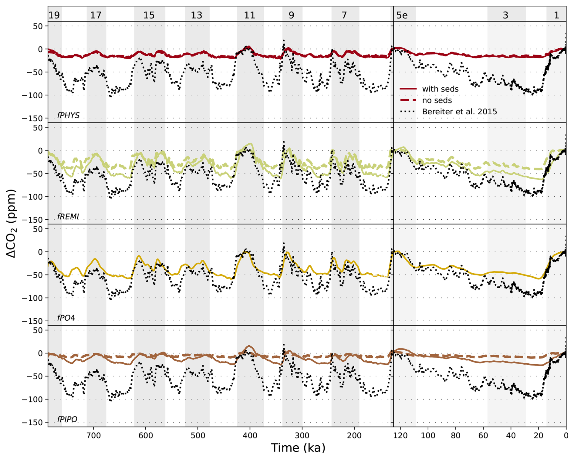
Figure 5 Transient variations in atmospheric CO₂ due to effects fPHYS, fPO4, fREMI, and fPIPO and reconstructed by Bereiter et al. (2015). Shown is the deviation from the pre-industrial value. Grey shading indicates uneven MIS as indicated at the top of the figure. Dashed lines denote runs without the sediment module (not available for PO4). The same plots for the other simulations are shown in Fig. S17.

3.2 Atmospheric CO₂

Interactive sediments have a negligible effect on the atmospheric CO₂ changes caused by physical forcings but largely alter the CO₂ change effect of biogeochemical forcings (Fig. 5). Marine CO₂ uptake and reduced export production due to physical forcings cause a net dissolution/reduced deposition of sedimentary CaCO₃ during glacials, and marine ALK and DIC build up as a consequence. A large fraction of the glacial DIC pool is eventually incorporated into CaCO₃ and deposited during deglaciations with little effect on outgassing. Under biogeochemical forcings, the larger CaCO₃ perturbations also have a larger effect on sea–air gas exchange. Another effect is the reduction in sedimentary organic carbon burial rates during interglacials in response to increased nutrient supply (fPO4) or a flattened remineralisation profile (fREMI) during glacial phases. Sedimentary POC accumulates during glacial phases and is subsequently remineralised during deglaciations, raising DIC and reducing ALK, both contributing to enhanced CO₂ outgassing. We explore the forcing-specific differences in more detail by focusing exemplarily on the last deglaciation.

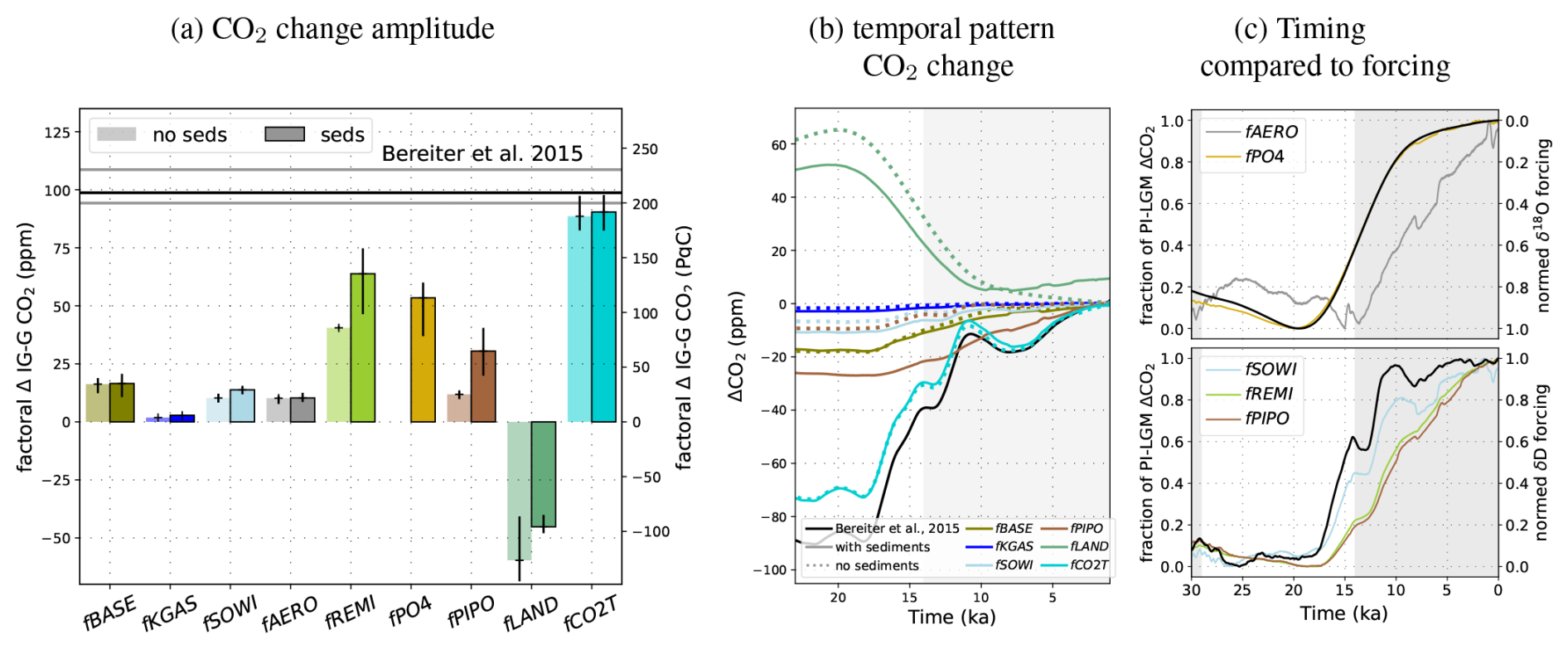
Figure 6 Effects of individual forcings on deglacial atmospheric CO₂ changes compared to reconstructions. Panel (a) shows the factorial contributions to the mean glacial–interglacial CO₂ amplitude over the last five glacial terminations (excluding terminations before the Mid-Brunhes transition) and the range between their minimum and maximum. Light colours indicate results without interactive sediments, and full colours indicate results with interactive sediments. The mean, minimum, and maximum amplitudes over the last five deglaciations in the ice core record (Bereiter et al., 2015) are shown by the black and grey horizontal lines. Panel (b) shows the factors discussed in the text transiently over the last termination. Panel (c) shows time lags between the factors and the respective forcing time series (black lines). The δ¹⁸O and δD forcings are taken from Lisiecki and Raymo (2005) and Jouzel et al. (2007) (see Methods).

By design, CO₂ restoring causes marine carbon uptake that fills the gap between dynamic atmospheric CO₂ changes in fBASE and reconstructions (Figs. 6, S6, S17), so here we focus on the other forcings. Biogeochemical forcings produce the largest CO₂ differences between the LGM and PI with regard to the reconstructions (Figs. 5, 6a). The weathering–burial disequilibrium, which builds up over the glacial phase under these forcings, amplifies the deglacial CO₂ rise, particularly in fREMI and fPIPO. In both cases, sedimentary accumulation of CaCO₃ spikes during deglaciation due to increased CaCO₃ export as the forcings wane (Fig. 2). The corresponding ALK reduction expels more CO₂ from the surface ocean into the atmosphere. In the case of fREMI, this is further enhanced by a reduction in sedimentary POC accumulation during the deglaciation, which reduces the carbon loss to the sediments. In both cases, the sedimentary processes that amplify the deglacial CO₂ rise also reduce its speed and smooth out transient features of the δD record which are translated into transient atmospheric CO₂ changes in simulations without interactive sediments (Fig. 6c). These time lags are caused by the strengthened export production, which counteracts carbon degassing, and a large buildup of ALK and DIC during the glacial phase (amplified by interactive sediments; Fig. S18), which is only gradually reduced by enhanced CaCO₃ burial during deglaciations (Fig. S19). If, instead, export production and sedimentary carbon accumulation decrease during the deglaciations due to increased nutrient limitation (fPO4), the carbon previously incorporated into biogenic matter is outgassed from the surface ocean, and no lag between CO₂ rise and the forcing emerges. Weathering–burial imbalances have a smaller effect on circulation-driven deglacial CO₂ degassing (fSOWI, fAERO), regarding both amplitude and timing. However, CO₂ also lags temperature in fAERO (with and without interactive sediments), due to the hysteresis of the AMOC. Enhanced Southern Ocean wind stress (fSOWI) is the only forcing in our simulation set that is able to create fast, transient CO₂ releases despite weathering–burial imbalances. In all simulations except LAND, the lowest CO₂ values occur during the coldest interval of glacial cycles, the glacial maxima (Figs. 5, S17). In all simulations in which the deglacial CO₂ rise lags that of temperature, CO₂ keeps rising throughout the Holocene.

Interactive sediments also affect the sensitivity of the deglacial CO₂ rise to peak interglacial warmth: only by including interactive sediments does our model simulate a shift in the MBT glacial–interglacial CO₂ amplitude comparable to the observations (Figs. S20, S21).

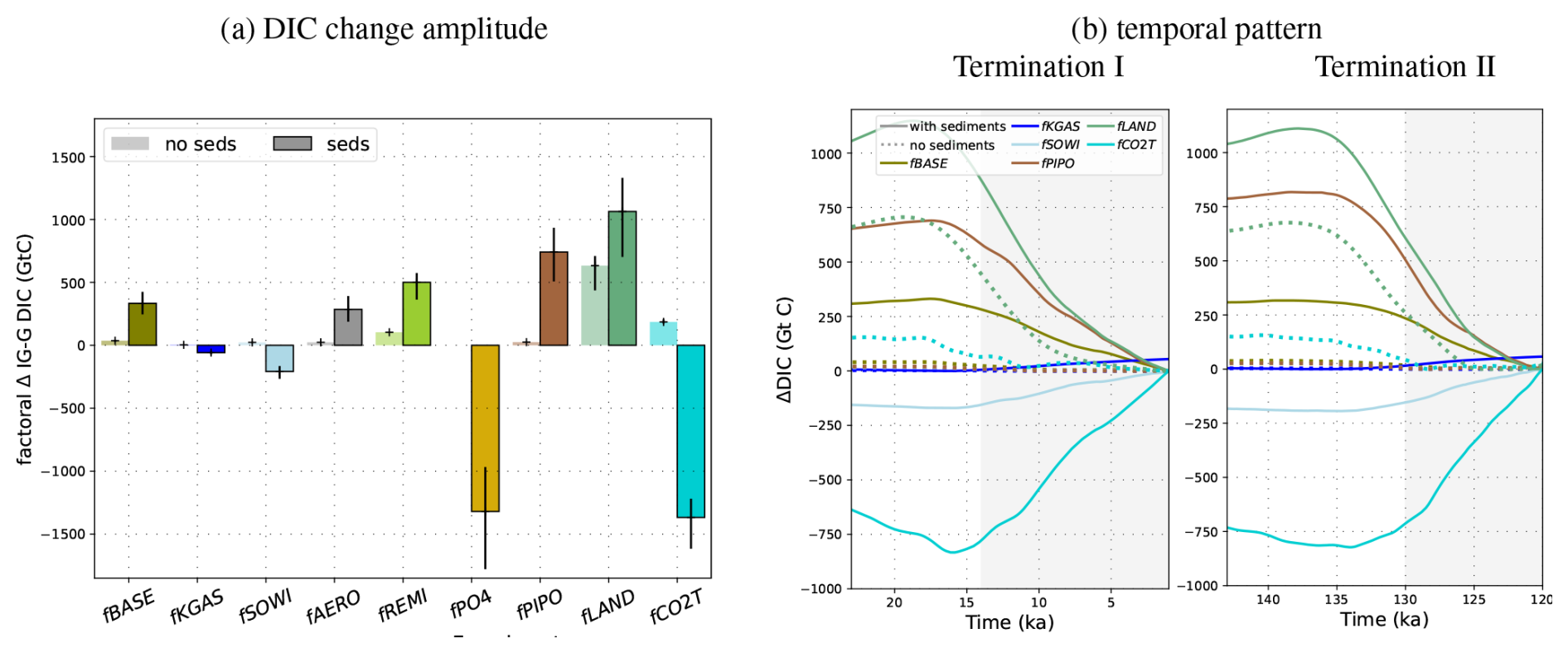
Figure 7 Factorial DIC concentration changes for each forcing over glacial cycles, from the highest or lowest DIC value during the glacial cycle, depending on which occurs earlier, to the other extreme. (a) Factorial contribution of each forcing to the mean DIC amplitude over the last five glacial cycles and the range between their minimum and maximum. Light colours show the contributions without dynamic sediments, and full colours show the contributions with dynamic sediments. In panel (b), the factorial contribution of selected forcings to the temporal DIC evolutions across two terminations is shown with and without interactive sediments.

3.3 Marine DIC and the surface carbonate system

Due to interactive sediments in our simulations, increased uptake or release of carbon in the surface ocean does not linearly correlate with DIC changes because marine carbon storage is also affected by changes in the deposition and dissolution fluxes of particulate carbon at the ocean–sediment interface. Interactive sediments affect marine carbon, ALK, and nutrient concentrations in two important ways: firstly, sediments form a large dynamic reservoir which can store and release large amounts of carbon and nutrients for hundreds to tens of thousands of years. Secondly, sedimentary mass accumulation, dissolution, and remineralisation rates control sedimentary burial, the only permanent sink for carbon and nutrients in our simulations and the only mechanism by which environmental change can create imbalances with the prescribed constant solute flux from land. Fluxes into and out of the sediments respond to environmental change, in some cases on the timescale of water mass replacement or regional productivity changes. Carbon fluxes from the sediments directly affect the ocean, but not the atmosphere, which causes different amplitudes in the simulated DIC and atmospheric CO₂ changes and different timings of carbon accumulation in the ocean and atmosphere. With interactive sediments, fBASE, fAERO, fREMI, fPIPO, and fLAND produce the highest DIC during glacial maxima and the lowest DIC during interglacials as altered air–sea gas exchange and sediment accumulation result in a net influx of carbon into the ocean during glacial phases. However, while altered air–sea gas exchange still draws down atmospheric CO₂ under fKGAS, fSOWI, and fPO4, larger changes to the sediment fluxes remove carbon from the glacial ocean (Fig. 2) and store excess carbon as carbonate and organic carbon in sediments instead of as DIC in the ocean. Consequently, the lowest DIC occurs during glacial maxima rather than during interglacials under these effects (Figs. S4, S5). fCO2T alters sedimentary carbonate preservation such that DIC extremes do not occur at the same time as atmospheric CO₂ extremes but in between; i.e. the DIC maximum occurs during glaciation, and the DIC minimum occurs during deglaciation (Fig. S6). Furthermore, the onset of the deglacial CO₂ rise in simulations with sediments does not always coincide with the onset of the deglacial DIC change, as is the case in simulations without sediments. This is simulated, for example, for terminations I and II due to fLAND and fCO2T (Fig. S23) and for terminations I, II, III, and IV due to fPO4 and fALL (Fig. S22). Across the tested processes, the corresponding ocean DIC inventory changes from glacial to interglacial are −1800–1400 GtC (Fig. 7), while the atmospheric inventory changes by −170–190 GtC (Fig. 6) over the same period. For individual processes, DIC changes differ by a factor of up to 28 between simulations with and without interactive sediments, while CO₂ changes in the atmosphere are maximally 4 times larger when interactive sediments are considered (Figs. 7, 6).

The magnitude of these DIC changes depends on the forcing strength, which varies between glacial cycles. The lukewarm interglacials of the first 350 kyr of our simulations do not restore the export fluxes and sedimentary CaCO₃ preservation required to compensate the prescribed solute influx, so marine DIC concentrations are persistently higher 800–450 ka than during the PI. Interglacials of the last 450 kyr of the simulation reduce DIC in the long term because they are warm and long enough for increased carbon transfer into sediments and sediment burial.

3.4 δ¹³C in the atmosphere and ocean

δ¹³C in the atmosphere and ocean is also affected by weathering–burial imbalances. Ice cores preserve the δ¹³C signature of atmospheric CO₂ (Friedli et al., 1984), which showed large fluctuations during the last glacial cycle (Fig. 8), such as fluctuations of ∼ 0.5 ‰ during MIS4 (71–57 ka) and during the last deglaciation (∼ 18–8 ka) (Eggleston et al., 2016). They also show a long-term increase in atmospheric δ¹³C across the last glacial cycle (Schneider et al., 2013; Eggleston et al., 2016). Reconstructions of δ¹³C changes in marine DIC show different trajectories in different ocean basins and water masses (Oliver et al., 2010; Peterson and Lisiecki, 2018). The δ¹³C signature of marine DIC in a given location and atmospheric CO₂ is influenced by processes which affect the whole marine carbon reservoir (e.g. changes in the amplitude and composition of marine carbon input or output fluxes) and by changes in water mass distribution, export production, and isotopic fractionation during sea–air gas exchange and primary production (Jeltsch-Thömmes et al., 2019; Jeltsch-Thömmes and Joos, 2023), with any signal diluted by the land biosphere. None of the forcings that we applied here produce all of the reconstructed features. However, they show the importance of considering weathering–burial imbalances in their interpretation.

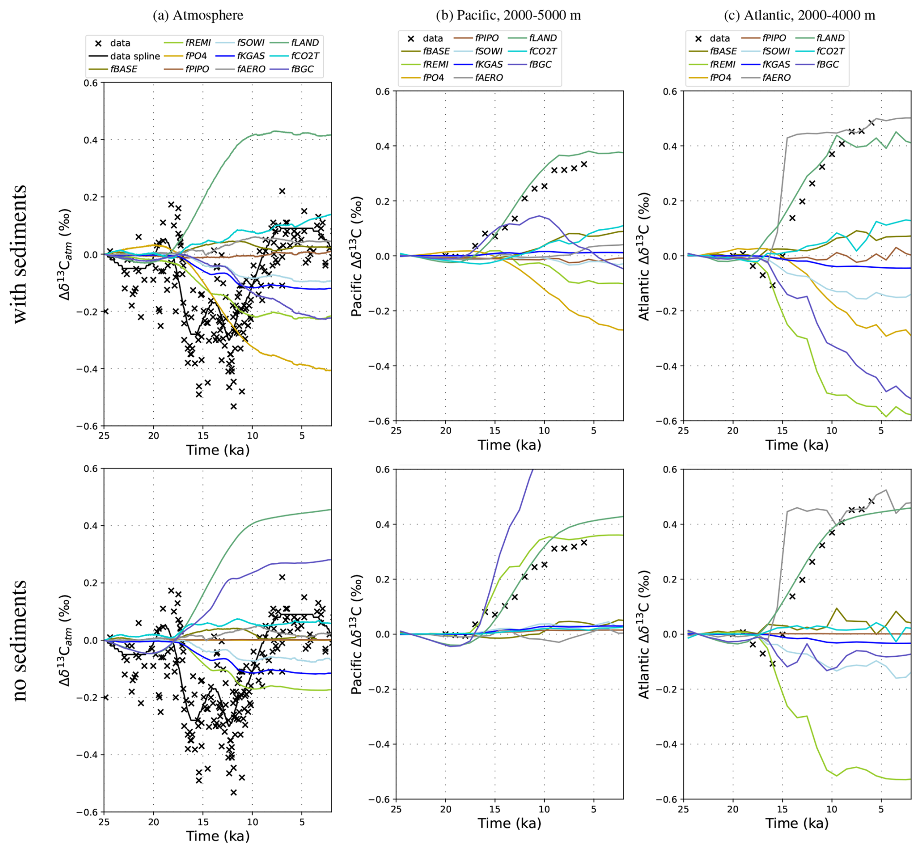
Figure 8 δ¹³C over the last deglaciation in (a) the atmosphere, (b) the deep Pacific (−35–55° N, 120–266° E), and (c) the deep Atlantic (0–65° N). Lines are simulation results. Crosses are reconstructions from Schmitt et al. (2012), Eggleston et al. (2016), and Peterson and Lisiecki (2018). All results are shown as differences from 24 ka. Results with interactive sediments are shown in the top row, and results without sediments are shown in the bottom row.

Figure 8 shows the factorial effects of the different forcings on atmospheric and marine δ¹³C across the last deglaciation in comparison to the reconstructed isotopic shifts in these reservoirs. Under fLAND, δ¹³C changes are driven by the simulated release of isotopically light land carbon (−24 ‰) during glacial inceptions and throughout the glacial, resulting in δ¹³C minima in all reservoirs during glacial maxima and large δ¹³C increases during deglaciation in response to land carbon uptake, with and without interactive sediments (Fig. 8). This whole-ocean shift is the dominant signal in δ¹³C records of the deep Pacific. In simulations without interactive sediments, fREMI also causes a similar shift in the deep Pacific, yet the shift is of opposite sign in simulations with interactive sediments due to the negative geological POC balance during the deglaciation (Fig. 2). fPO4 has a similar isotopic effect on the ocean to fREMI with sediments because it also leads to the release of sedimentary organic carbon during the deglaciation. Since the processes that affect δ¹³C${}_{{\mathrm{CO}}_{\mathrm{2}}}$ and δ¹³C_DIC are different, and δ¹³C_DIC varies between ocean basins, the forcings which best reproduce reconstructed evolution of δ¹³C also vary between atmosphere and ocean and specific water masses (Oliver et al., 2010). This indicates that different processes were likely the dominant controls on δ¹³C regionally, even if they were not necessarily the dominant drivers of atmospheric CO₂. The impact of interactive sediments also varies between water masses. For example, in the deep Pacific, accumulation of isotopically light δ¹³C as in fLAND likely dominated (Fig. 8b) but must have over-compensated the sediment-enhanced isotopic effects of fREMI and fPO4 and cannot explain the reconstructed CO₂ rise (Fig. 6). In the deep North Atlantic, the magnitude of the δ¹³C shift can also be reproduced by additional radiative cooling and the resulting AMOC shoaling due to fAERO (Fig. 8c), and the simulated isotopic shifts are less affected by interactive sediments.

In the atmosphere, the largest δ¹³C variability (up to ± 0.5 ‰) is also produced by fLAND, with and without interactive sediments, and by fREMI and fPO4 in simulations with interactive sediments. In fact, the gradual trend in reconstructed atmospheric δ¹³C over the last glacial cycle ($+\sim$ 0.5 ‰ from inception to LGM) is only achieved in fPO4, the forcing with the biggest effect on sedimentary organic carbon storage (Fig. 2). fLAND causes similar long-term changes but of the opposite sign. No simulation captures the large millennial-scale fluctuations in the reconstructions (Fig. 8). Given our smoothed forcing and the absence of freshwater forcings, our simulations do not contain realistic millennial-scale circulation changes, which would likely be required to simulate these fluctuations (Tschumi et al., 2011; Schmitt et al., 2012; Menviel et al., 2015). It is well established that a complex combination of processes is required to explain the atmospheric δ¹³C record (e.g. Menviel et al., 2015), but a simulation over the last glacial period or the deglaciation accurately reproducing the reconstructions has not yet been achieved, and reconciling reconstructed with simulated atmospheric δ¹³C remains a major challenge for future work. However, our simulations show that interactive sediments change the δ¹³C signals of Earth system changes on deglacial timescales and need to be considered in future work, despite challenges associated with model spin-up, as discussed next.

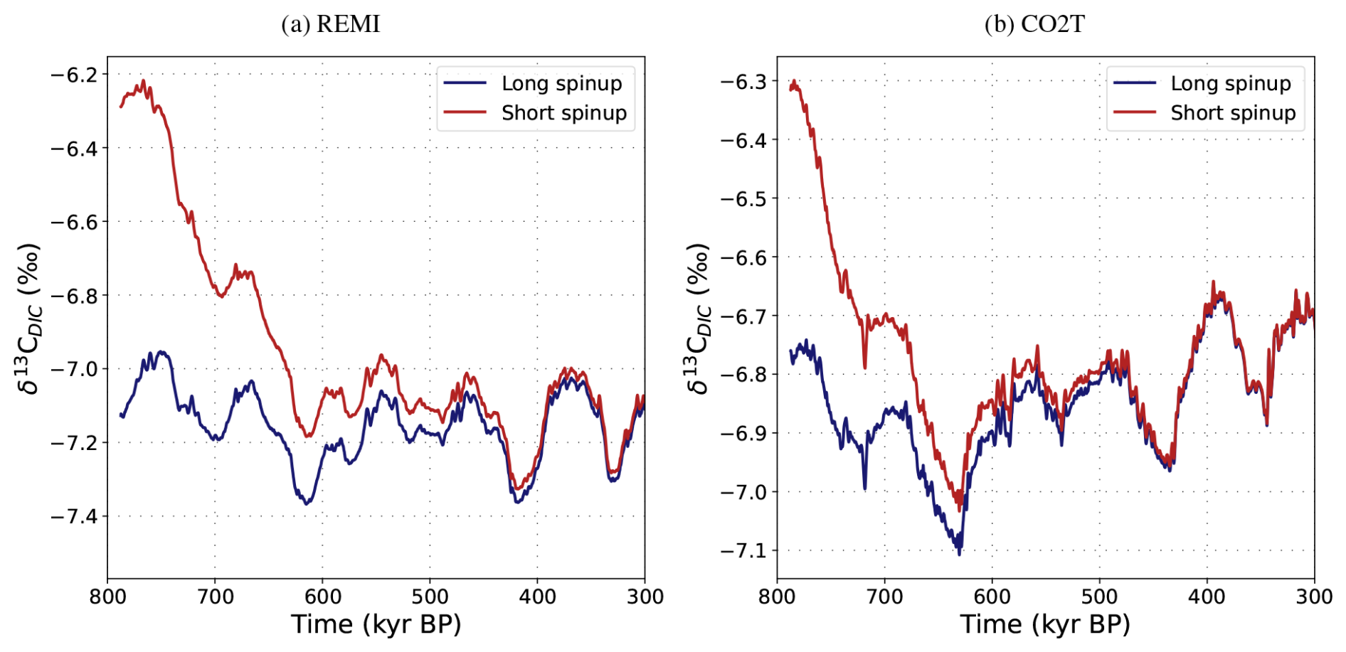
Figure 9 Comparison of simulated atmospheric δ¹³C in simulations REMI and CO2T when started from a “short spin-up”, i.e. a 70 kyr PI spin-up followed by a 2 kyr adjustment to MIS19 conditions, and a “long spin-up”, i.e. the short spin-up plus 215 kyr of transiently simulated MIS19–MIS15.

3.5 Long isotopic drifts due to weathering–burial imbalances

An important technical lesson of our simulations is that the long adjustment timescale in the geologic carbon cycle also presents an initialisation problem, especially for carbon isotopes (Jeltsch-Thömmes and Joos, 2023). We started our experiments from MIS19, which was a colder interglacial than the Holocene, and Holocene conditions were not reached during the lukewarm interglacials of the first 400 kyr of the simulations. In simulations with interactive sediments, the initial imbalance between weathering inputs derived from the pre-industrial spin-up and burial fluxes adjusting to the colder lukewarm interglacials and glacial states caused δ¹³C drifts during the first glacial cycles (Fig. 9). Consequently, the simulated glacial–interglacial δ¹³C signal over this period is altered by the long-term adjustment of the geologic carbon cycle. We addressed this issue by transiently simulating two full glacial cycles before starting the experiments. The magnitude of the initial imbalance in the geologic carbon cycle, and hence isotopic drift, depended on the simulated forcing and was largest in simulations REMI, PIPO, and CO2T. Importantly, the drift is a result of perturbing the sediment–weathering balance. The drift can therefore not be corrected for with a control simulation without forcing because it only appears in the perturbed system. Instead, to avoid a drift, the experiment needs to start from an isotopically balanced geologic carbon cycle, which most commonly will require a long spin-up with a fully coupled open system, ideally over several glacial cycles, especially when simulating large changes in the biological pump or marine carbonate system. We suggest that the size of the transient imbalance of the geologic carbon cycle, and thus the length of the required spin-up, could be minimised by balancing the geologic carbon cycle not for an interglacial state but for the mean burial fluxes over a full glacial cycle.

Table 2 Quantified metrics of the carbon cycle according to reconstructions and model responses in our set of simulations with sediments. Shown are the factorial effects of the tested forcings and their non-linearities in comparison with reconstructed differences (LGM minus Holocene) over the last deglaciation (specific times of the comparisons vary slightly by proxy record, depending on temporal resolution and record length, and are indicated in the table header) in various proxy systems. The data references are provided at the bottom of the table. The direction of each arrow indicates whether a difference is positive (pointing upwards, teal) or negative (pointing downwards, brown). The width of the arrows shows the size of the difference relative to the reconstruction in the uppermost row, “Data”. For POM export, only qualitative reconstructions exist. Hence, the arrows showing simulated effects are normed by the biggest effect of any forcing.

4 Discussion

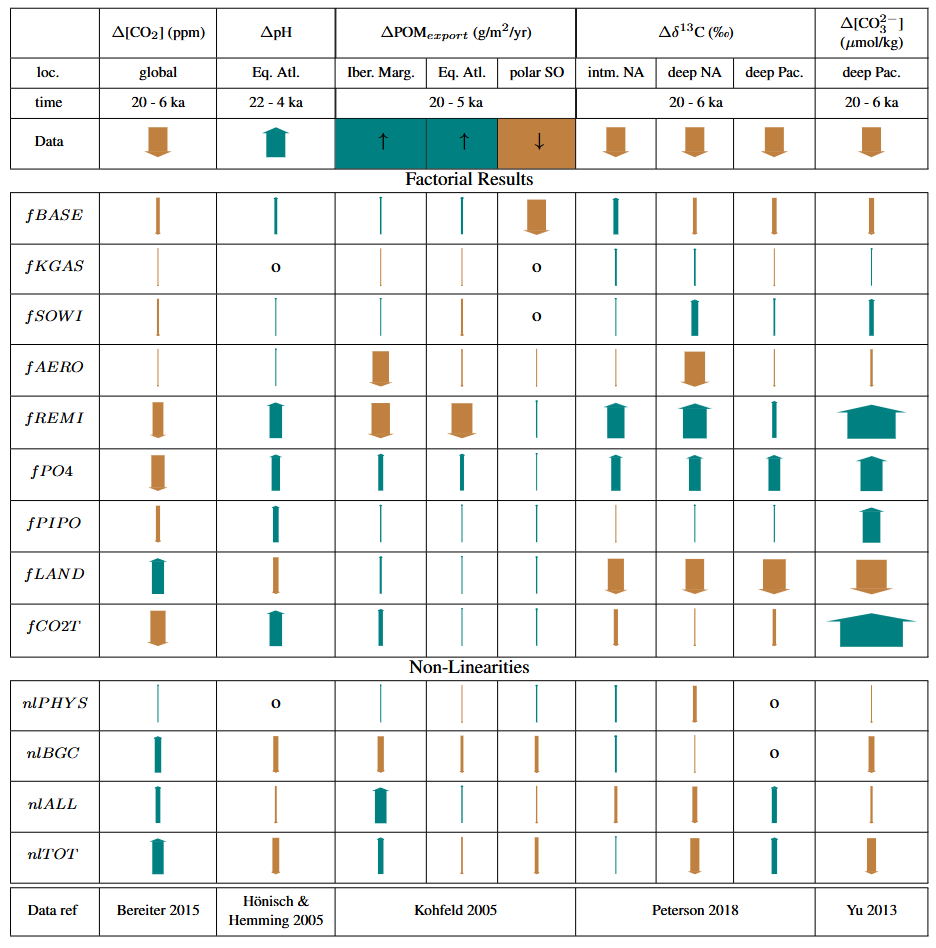
Table 2 provides an overview of different proxy signals that are produced by our factorial forcings and the non-linearities that arise when they are combined, with interactive sediments over the last deglaciation. The first row shows the reconstructed direction of LGM–Holocene differences, and the next lines show the direction and relative size (compared to the proxy signal) of changes induced by the various tested forcings. The last four rows show the direction and relative size of non-linearities caused by three different combinations of the forcings above. For many of the considered proxies, the signals are strongly amplified by the dynamic weathering–burial imbalances and the non-linearities are larger with than without interactive sediments. However, the non-linearities are still small compared to the effect of individual biogeochemical forcings and for some proxies are of a similar size to the effect of physical forcings. Hence, in most cases, proxy changes provide a first-order constraint on the plausibility of large changes in individual processes. fBASE, the effect of temperature changes due to orbital, albedo, and greenhouse gas changes, moves almost all proxy systems in the reconstructed direction (the directions of the arrows match) but almost never to the reconstructed extent (the widths of the arrows do not match). It is only sufficient to explain strongly reduced export production in the polar Southern Ocean at the LGM, which in our model is predominantly driven by surface cooling and sea ice expansion regardless of which other processes also occurred.

We identified two processes by which weathering–burial imbalances most effectively raise atmospheric CO₂ during deglaciations in our simulations: ALK removal and organic carbon remineralisation. Under fPIPO and fREMI, the combination of high ALK at the end of glacial phases and increased CaCO₃ export production during deglaciation causes large transient CaCO₃ deposition events in the open ocean (Fig. 2) which remove the excess glacial ALK and thus drive a large but slow continuous CO₂ rise compared to the reconstruction. The marine DIC and ALK that built up over the previous glacial phase are too large to be removed instantly, and the resulting large deposition of CaCO₃ during the deglaciation persists far into the interglacial. In consequence, these forcings produce poorer model–data matches for Holocene CaCO₃. We also showed that the resulting δ¹³C and [CO${}_{\mathrm{3}}^{\mathrm{2}-}$] signals in the deep Pacific are not consistent with reconstructions. fCO2T shows the effect of forced ALK removal during glaciations to reproduce the reconstructed atmospheric CO₂ record and can serve to study the effect of ALK removal through means other than deep-ocean CaCO₃ burial (e.g. shallow deposition, coral reef growth, reduced terrestrial input) on other proxy systems. This forcing causes deep-ocean CaCO₃ dissolution and increasing marine DIC during the deglaciation, moving δ¹³C in the deep Pacific in the proxy-consistent direction but still producing a large mismatch in [CO${}_{\mathrm{3}}^{\mathrm{2}-}$]. fPO4 results in a deglacial CO₂ rise due to a reduction in export production and increased remineralisation of sedimentary organic matter which accumulated during the previous glacial period under reduced benthic O₂ concentrations. The resulting CO₂ increase is of a similar amplitude to that due to fREMI but happens faster, more consistent with the reconstruction. In addition, deep Pacific [CO${}_{\mathrm{3}}^{\mathrm{2}-}$] is less perturbed by this effect than by fREMI or fCO2T, yet deep-ocean δ¹³C is shifted in the wrong direction. Future work will have to test which combinations of these processes are most consistent with the wide range of available proxy data.

It is well established that cooling and circulation changes altered sea–air gas exchange and increased deep ocean carbon storage by isolating it from the surface during glacial phases (e.g. Brovkin et al., 2007). Combined, these effects contribute to changes in atmospheric CO₂ in our simulations that are comparable to Brovkin et al. (2012) (26 ppm compared to 30 ppm).

Isolating the deep Pacific through reduced Southern Ocean wind forcing (effect fSOWI) caused a glacial CO₂ decline by ∼ 13 ppm, the biggest CO₂ drawdown on top of the effect orbital cooling (fBASE) of any isolated physical forcing that we tested. Tschumi et al. (2011) showed that this effect also has the potential to cause larger CO₂ drawdown with sedimentary amplification than simulated here. The idealised strong reductions in wind speeds over the Southern Ocean prescribed by Tschumi et al. (2011) as a tuning knob for producing old deep-ocean waters are unrealistic, but other processes could have contributed to increased isolation of the deep Pacific. Bouttes et al. (2011) showed that, during glacial stages, enhanced brine rejection during sea ice formation can isolate abyssal waters and cause atmospheric CO₂ and δ¹³C changes that are similar to those reconstructed. Enhanced brine rejection could thus have provided an additional physical process that increased the glacial marine carbon storage. The strength of this process, however, is only poorly constrained, and Ganopolski and Brovkin (2017) showed that, at a sufficient strength to significantly affect deep-ocean carbon storage, this process creates bigger Δ¹⁴C anomalies in the deep ocean than reconstructed. Following Menviel et al. (2011), they also argue that the timing of increased sea ice formation and atmospheric CO₂ changes during the last deglaciation (Roberts et al., 2016) is not entirely consistent with a strong control of brine formation rates on marine carbon storage.

In further agreement with other modelling studies, e.g. Buchanan et al. (2016) and Morée et al. (2021), we find that changing the efficiency of the biological pumps (fREMI) is an efficient mechanism to achieve glacial–interglacial atmospheric CO₂ changes similar to those reconstructed from ice cores. However, because of its large effects on deep Pacific [CO${}_{\mathrm{3}}^{\mathrm{2}-}$] and CaCO₃ accumulation during deglaciation, it was unlikely the dominant carbon cycle change over the last glacial cycle.

A relevant role of marine sediments, particularly sedimentary CaCO₃, in glacial–interglacial carbon cycle dynamics has long been discussed (e.g. Broecker, 1982b; Broecker and Peng, 1987; Opdyke and Walker, 1992; Archer and Maier-Reimer, 1994; Raven and Falkowski, 1999) and shown in numerical experiments of differing physical and biogeochemical complexities (Ridgwell et al., 2003; Joos et al., 2004; Tschumi et al., 2011; Menviel et al., 2012; Roth et al., 2014; Wallmann et al., 2016; Ganopolski and Brovkin, 2017; Jeltsch-Thömmes et al., 2019; Köhler and Munhoven, 2020; Stein et al., 2020; Kobayashi et al., 2021). In agreement with other studies (e.g. Ganopolski and Brovkin, 2017; Köhler and Munhoven, 2020), we find that changing marine ALK can produce large CO₂ changes. Organic carbon storage is less often considered in modelling studies, although it also showed significant changes across the last glacial cycle (Cartapanis et al., 2016). Out of the forcings we tested, reduced nutrient limitation during glacial phases (fPO4) produces temporal and regional organic carbon deposition changes that were most consistent with the reconstructions. In this simulation, marine sediments turn into a strong carbon sink during cold phases. The simulated increased organic carbon deposition during glacial phases reproduces the reconstructed long-term trends in atmospheric and surface ocean δ¹³C during glacials, but it is not sufficient in isolation to reproduce the reconstructed deep-ocean δ¹³C changes in the Pacific and Atlantic. Thus, while sedimentary organic carbon burial could have provided a carbon sink during glacial phases, it must have been operating alongside other processes to allow for the reconstructed benthic δ¹³C evolution. Interestingly, processes that increase organic carbon burial during glacial phases (fPO4, fREMI) show that some of the deposited organic carbon can be returned to the ocean during deglaciations with a large potential to contribute to a fast post-glacial rise in atmospheric CO₂. In addition to carbon, nutrients are also removed from the ocean when organic matter is buried (Roth et al., 2014). Tschumi et al. (2011) demonstrated in their steady-state experiments that increased organic nutrient burial enhances nutrient limitation on export production and reduces CaCO₃ export, which increases surface ALK and amplifies the CO₂ drawdown caused by the increased burial of organic carbon. Under fREMI, this process operates transiently. Given the reconstructed increased organic carbon burial rates during glacial maxima, this could have been a relevant process over the last glacial cycles, though it might have been reduced in its efficiency by reductions in the PIC : POC of export production during glacial phases (Dymond and Lyle, 1985; Sigman and Boyle, 2000). Finally, sedimentary organic carbon oxidation can also regulate marine ALK by affecting sedimentary CaCO₃ dissolution (Emerson and Bender, 1981; Sigman and Boyle, 2000), but this effect is not directly quantified in our setup. However, we can assess that increased sedimentary organic matter remineralisation on a global scale during glacial phases does not occur due to any of our tested forcings. On the contrary, the effects (fPO4, fREMI) that increase organic carbon burial during glacial maxima, a prominent feature of the reconstructions, decrease globally averaged sedimentary remineralisation rates during glacial times.

A close relationship between DIC and Δ¹⁴C(DIC) is found in modern deep-ocean waters, and this relationship has been used to reconstruct past DIC changes from radiocarbon reconstructions (Sarnthein et al., 2013). Sedimentary carbon fluxes can decouple deep-ocean Δ¹⁴C from DIC (Dinauer et al., 2020) and change DIC without altering sea–air carbon transfer, meaning that DIC changes do not necessarily imply a comparable CO₂ change in the atmosphere. In all of our simulations with interactive sediments, the DIC inventory change over a glacial cycle is larger than the simultaneous atmospheric CO₂ inventory perturbation because of changes in carbon reservoirs in sediments and weathering–burial imbalances. Changes in the simulated sedimentary burial fluxes result in net transfers of up to 2000 PgC between the carbon pools of the ocean and sediments throughout a glacial cycle, while the net loss of atmospheric carbon to reproduce the reconstructed glacial CO₂ is roughly 200 PgC (Sigman and Boyle, 2000; Yu et al., 2010) and the net loss of terrestrial carbon is on the order of 500–1000 PgC (Jeltsch-Thömmes et al., 2019). The carbon cycle impact of glacial cycles was thus likely larger in the ocean than in the atmosphere (Roth et al., 2014; Buchanan et al., 2016), due to changes in sedimentary carbon storage. In some of our simulations, large DIC changes are produced by big sustained weathering–burial imbalances during glacials that cannot be compensated during the relatively short deglaciations and cause interglacial carbonate preservation patterns that are not consistent with observations (Figs. S11, S12). While such simulated scenarios are thus unrealistic, it does not generically preclude the possibility of large transient weathering–burial imbalances during glacial phases. Testing a wider range of forcing magnitudes and combinations with the same model but different setup, Jeltsch-Thömmes et al. (2019) (the DIC results of which are published in the Appendix of Morée et al., 2021) found a larger DIC change between the pre-industrial and the LGM than simulated here (3900 ± 550 GtC compared to a maximum of 1100 ± 300 GtC in Fig. 7) that is consistent with carbonate system proxy constraints. Combinations of the tested forcings thus allow larger transient weathering–burial imbalances than produced by our simulation ensemble that can still be reconciled with carbon cycle proxies. Some of the tested forcings also show lower glacial than interglacial DIC (fPO4, fCO2T), showing that CO₂ removal from the atmosphere in theory does not need to result in increased DIC in the ocean. Instead, these biogeochemical forcings cause sedimentary changes that can store large amounts of carbon in inorganic and organic sedimentary matter. Kemppinen et al. (2019) and Jeltsch-Thömmes et al. (2019) previously showed and discussed the possibility of a negative glacial DIC anomaly due to increased sedimentary storage. As found by Jeltsch-Thömmes et al. (2019), organic carbon burial extensive enough to cause a negative glacial DIC anomaly (e.g. fPO4) produces large δ¹³C signals of opposite sign than reconstructed and thus seems unlikely. In the study by Jeltsch-Thömmes et al. (2019), a negative glacial DIC anomaly due to ALK-driven CaCO₃ accumulation is also inconsistent with the proxy record of the last 25 kyr. Consistently, we find that reconstructed deep Pacific [CO${}_{\mathrm{3}}^{\mathrm{2}-}$] changes make a large-scale ALK-driven (fCO2T) glacial CaCO₃ accumulation, which reduces atmospheric CO₂ while also reducing DIC, which is unlikely because it causes larger deep Pacific [CO${}_{\mathrm{3}}^{\mathrm{2}-}$] changes than reconstructed over the last deglaciation (Table 2). The isotopic signal of such large CaCO₃ deposition, however, is smaller than that of POC burial changes and could more likely be overprinted by other processes (e.g. terrestrial carbon release and export production changes) to yield proxy-consistent evolutions (Table 2).

It has long been suggested that sedimentary imbalances also contributed to the reconstructed interglacial sedimentary changes and CO₂ rises after deglaciations (Broecker et al., 1999; Ridgwell et al., 2003; Joos et al., 2004; Broecker and Stocker, 2006; Elsig et al., 2009; Menviel et al., 2012; Brovkin et al., 2016). Consistently, we find that CO₂ degassing from the ocean persisted throughout deglaciations and into interglacials (e.g. Brovkin et al., 2012) and that the carbon cycle does not reach a new equilibrium before the next glacial inception (e.g. supply–burial imbalances in the late Holocene in Table S2). In our simulations, AMOC hysteresis, sedimentary changes, and delayed temperature responses, e.g. due to ice sheets (mimicked by scaling most forcings to the δ¹⁸O record), introduce memory effects which buffer deglacial carbon cycle reorganisations and cause continued CO₂ rise throughout interglacials. For example, in PO4, BGC, and ALL, the simulations which best align with the reconstructed glacial–interglacial organic carbon burial changes, not all glacial organic matter is remineralised and carbonate dissolution continued throughout the interglacials.

5 Conclusions

In response to different simulated carbon cycle forcings over the repeated glacial–interglacial cycles of the past 780 kyr in the Bern3D model, we found large sedimentary changes which substantially alter marine carbon and nutrient concentrations and spatial distributions. Our simulations show that biogeochemical forcings are required to perturb the sediments sufficiently to reproduce reconstructed burial changes and CO${}_{\mathrm{3}}^{\mathrm{2}-}$ variations, yet compensating processes (e.g. shallow carbonate deposition) must have operated to reduce the buffering impact of this sedimentary perturbation on the deglacial carbon cycle reorganisation in order to match the speed of the associated carbon release. These results have implications for model experiment design and the interpretation of δ¹³C proxy data: we showed that the long timescales of ocean–sediment interactions and the weathering–burial cycle pose substantial challenges for model spin-up because imbalances in the geologic carbon cycle can cause isotopic drifts at the beginning of simulations and which are not present in a control run. Depending on the initial isotopic imbalance, it takes up to 200 kyr for the drift to subside and the signal of the applied forcing to dominate the simulated transient δ¹³C changes. Further studies are needed to test whether δ¹³C can be spun up in more computationally expensive models by combining them with lower-complexity models. In the absence of such a spin-up strategy, open-system simulations of glacial δ¹³C are likely strongly affected by these initial drifts severely hampering interpretation of results. These long adjustment timescales also pose challenges for separating long-term from short-term signals in the proxy records.

In terms of glacial carbon cycle dynamics, our set of factorial simulations leads to the following conclusions.

Firstly, ocean–sediment interactions and related weathering–burial imbalances, including fluxes of nutrients, alkalinity, and organic and inorganic carbon, tend to amplify glacial–interglacial CO₂ change.

Secondly, the relationship between marine DIC and atmospheric CO₂ changes is not linear across the different forcings and is strongly influenced by sediment fluxes. For example, the potential addition of phosphate from exposed continental shelves causes a decrease in atmospheric CO₂ and marine DIC by increasing sedimentary carbon storage. Factorial simulations yield changes in the ocean DIC inventory between −1340 to +1400 GtC and in the atmospheric CO₂ inventory between −96 and 180 GtC (−45 and 80 ppm) over the last five deglaciations in response to individual prescribed physical and biogeochemical forcings. This suggests that approaches utilising the relationship between radiocarbon and DIC from modern data to reconstruct the ocean's glacial DIC inventory and the postulated corresponding CO₂ change from glacial radiocarbon data may be biased.

Thirdly, ocean–sediment interactions strongly impact the evolution of important carbon cycle parameters such as δ¹³C(DIC) and δ¹³C${}_{{\mathrm{CO}}_{\mathrm{2}}}$, CO${}_{\mathrm{3}}^{\mathrm{2}-}$, export production, CaCO₃ and POM burial fluxes, preformed and remineralised nutrient concentrations, and oxygen. The interpretation of the proxy records without consideration of weathering–burial imbalances and ocean–sediment interactions for both organic and inorganic carbon may lead to erroneous conclusions.