Testing the reliability of global surface temperature reconstructions of the Last Glacial Cycle with pseudo-proxy experiments

Reconstructions of past variations in the global mean surface temperature (GMST) are used to characterise the Earth system response to perturbations and to validate Earth system simulations. Beyond the instrumental period, reconstructions rely on local proxy temperature records and algorithms aggregating these records. Here, we propose to establish standards for evaluating the performance of such reconstruction algorithms. Our framework relies on pseudo-proxy experiments (PPEs). That is, we test the ability of an algorithm to reconstruct a simulated GMST, using artificially generated proxy data created from the same simulation. We apply the framework to an adapted version of the GMST reconstruction algorithm used in Snyder (2016) and the metadata of the synthesis of marine proxy records for the temperature of the last 130 kyr from Jonkers et al. (2020). We use an ensemble of four transient simulations of the Last Glacial Cycle (LGC) or the last 25 kyr for the pseudo-proxy experiments.

Given the dataset and the algorithm, we find that the reconstruction is reliable for timescales longer than 4 kyr during the last 25 kyr. However, beyond 40 kyr BP, age uncertainty limits the reconstruction reliability to timescales longer than 15 kyr. For the long timescales, uncertainty on temperature anomalies is caused by a factor that re-scales near-global-mean sea surface temperatures to GMST, the proxy measurements, the specific set of record locations, and potential seasonal biases. Increasing the number of records significantly reduces all sources of uncertainty but the scaling. We also show that a trade-off exists between the inclusion of many records, which reduces the uncertainty on long timescales, and of only records with low age uncertainty, high accumulation rate, and high resolution, which improves the reconstruction of the short timescales.

Finally, the method and the quantitative results presented here can serve as a basis for future evaluations of reconstructions. We also suggest future avenues to improve reconstruction algorithms and discuss the key limitations arising from the proxy data properties.

1 Introduction

The global mean surface temperature (GMST) is a fundamental quantity to describe climate change. It is a major component of the Earth's energy balance and describes the response of the Earth system to external perturbations. Furthermore, the GMST is one of the variables characterising Earth's habitability and how ecosystems develop. Hence, GMST is the main target measure of international efforts to limit anthropogenic global warming (UNFCCC, 2015). The past evolution of GMST is used to evaluate Earth system models (ESMs; e.g. PAGES 2k Consortium, 2019; Brierley et al., 2020; Kageyama et al., 2021; Lunt et al., 2021) and to estimate the equilibrium climate sensitivity, i.e. the response of GMST to a doubling of atmospheric CO₂ concentrations (Snyder, 2016; Friedrich and Timmermann, 2020).

Comprehensive ESMs are being developed to project climate change for the end of the century and beyond. Some of these ESMs include an atmosphere–ocean general circulation model along with modules for ice sheets (Nowicki et al., 2016; Ziemen et al., 2019; Muntjewerf et al., 2020), iceberg melting (Rackow et al., 2017; Erokhina and Mikolajewicz, 2024), dynamic vegetation (Song et al., 2021), and the carbon cycle (Brovkin et al., 2012; Arora et al., 2020; Kleinen et al., 2021). During the Last Glacial Cycle (LGC; the last 130 kyr, which includes the Last Interglacial (LIG), the Last Glacial Period, and the Holocene), large changes in these Earth system components occurred in response to radiative forcing changes of comparable magnitude to those projected in future scenarios. Therefore, the LGC is an important evaluation period for ESMs.

Reconstructing past GMST relies on proxy records extracted for example from sediments or ice. Many methods for reconstructing the GMST over the LGC use a bottom-up approach, where many local proxy temperature records are combined to compute an area-averaged temperature (e.g. Shakun et al., 2012; Snyder, 2016; Friedrich and Timmermann, 2020; Osman et al., 2021; Clark et al., 2024). This approach aims to suppress noise and regional influences in these time series but remains sensitive to the spatial and temporal coverage of the data.

To our knowledge, a proper evaluation of such reconstruction methods has not been performed, which limits their use for model evaluations. In particular, we note several open questions regarding the quality of GMST reconstructions of and beyond the LGC:

• How reliable are GMST reconstructions of the LGC?

• Does the non-uniform spatiotemporal distribution of proxy samples lead to biased GMST reconstructions?

• Which sources of uncertainty impact reconstructions and in what way?

• What is the shortest timescale on which amplitudes and timings of GMST variations can be accurately reconstructed for a given algorithm and dataset?

• What are the sources of the loss of accuracy on short timescales?

• Which limiting factors should be prioritised for improving the GMST reconstruction quality (uncertainty, resolution)?

This study tests a reconstruction method similar to the one published in Snyder (2016, hereafter S16). This algorithm was used to compute a GMST reconstruction of the Pleistocene based on sea surface temperature (SST) proxy records to investigate glacial cycles. It is robust enough to tackle and account for the non-stationarity of climate states and the sparsity of the records. Compared to other algorithms proposed to reconstruct GMST on glacial–interglacial timescales, it quantifies uncertainties more comprehensively and has a limited reliance on model output. Therefore, we use it as the basis of our work, although most of the findings will likely hold for other algorithms using similar principles for the reconstruction.

This study does not provide a new reconstruction but an evaluation method based on pseudo-proxy experiments (PPEs) and transient climate simulations. PPEs enable the testing of an algorithm in controlled, idealised environments, where the underlying truth is known (i.e. the simulation outputs). They rely on pseudo-proxies that are synthetic time series imitating proxy records, based on the spatiotemporal climate state of the simulation. The computation of pseudo-proxies is performed using a proxy system model (sedproxy; Dolman and Laepple, 2018), which simulates the processes from the fixation of the climate-dependent quantity to the measurement of the proxy in the lab, including the entailed uncertainties. To create realistic pseudo-proxies, we use the metadata of a recently published database: the PalMod 130k marine palaeoclimate data synthesis (Jonkers et al., 2020, hereafter J20). This database provides numerous proxy records of near-surface sea temperature from marine sediments. It is metadata-rich, which enables us to test the impact of various uncertainty sources on the reconstruction and whether these are well accounted for in the algorithm's uncertainty estimates.

In the following, we first describe the J20 database and the transient climate simulations employed to compute the pseudo-proxies. Then, we present the GMST reconstruction algorithm and the design of the PPEs. The results from the PPEs follow this. Finally, we discuss the algorithm's performance when using the J20 metadata and future avenues to improve GMST reconstructions.

2 Data

2.1 Temperature reconstructions

Our study relies on one of the largest syntheses of marine proxy records for temperature of the LGC available: the extended PalMod 130k marine palaeoclimate data synthesis, beta version 2.0.0 (Jonkers et al., 2020, hereafter J20). This dataset is a multi-proxy compilation of globally distributed marine proxy records spanning the last 130 kyr and was developed within the PalMod initiative (https://www.palmod.de, last access: 16 January 2025; Latif et al., 2016; Fieg et al., 2023) as a comprehensive reference for transient climate simulations. We use various metadata from this database: core locations, proxy types, species (for $\mathrm{Mg}/\mathrm{Ca}$), sedimentation rates, and age ensembles. We prefer this database over the one assembled for S16, where only locations, proxy types, and mean chronologies are available. In particular, the effect of bioturbation can be computed using sedimentation rates or the impact of habitat preferences using species. The J20 database also provides a unified framework for the age models. These are constrained using a blend of radiocarbon dates (between 0 and ∼40 kyr BP) and δ¹8O benthic stratigraphy based on Lisiecki and Stern (2016). Chronological uncertainty is assessed using the Bayesian framework BACON (Blaauw and Christen, 2011). Specifically, the database contains 1000 age ensemble members for each sediment core. We do not use the temperature records in J20, as our study does not aim to present a new GMST reconstruction.

We selected all proxy records for SST located within the latitudes 60° N and 60° S, following S16, with at least 10 values. This leaves us with 265 time series at 189 locations. These records rely on temperature dependencies of the chemical composition, chemical product, and the temperature preferences of various organisms living near the sea surface. Here, this includes alkenone indices ($U_{\mathrm{37}}^k$, $U_{\mathrm{37}}^{k^{\prime }}$; 89 time series;  Prahl et al., 1988), a lipid-based index (TEX₈₆; 6 time series; Schouten et al., 2002), the long chain diol index (LDI; 4 time series;  Rampen et al., 2012), $\mathrm{Mg}/\mathrm{Ca}$ ratios in planktonic foraminifera (103 time series; Nürnberg et al., 1996), and microfossil assemblages (planktonic foraminifera, radiolaria, and diatoms; 63 time series;  Imbrie, 1971). In addition, we only kept the time series for which the representative season was indicated as annual (105 time series) or unspecified (112 time series). In some cases, assemblages from the same core are used to estimate winter and summer temperatures. If the time step coincides, we average the two to form 48 “pseudo-annual” time series.

Record metadata show some distinctive features (Figs. 1 and 2). Firstly, record locations tend to better cover the Atlantic than the Indian and Pacific oceans and tend to be close to the coast (Fig. 1-A). Secondly, the number of proxy records is maximum for the deglaciation (>200), while it is relatively constant between 40 and 120 kyr BP (82; Fig. 2a). However, substantial data gaps occur in the Southern Hemisphere for periods prior to the LGM (Fig. 1b). Thirdly, the lowest age uncertainty is achieved in the last 30 kyr (<3 kyr), where radiocarbon dating is reliable and frequently employed. For the rest of the LGC, median age uncertainty is slightly below 10 kyr. Finally, the highest temporal resolution and the highest accumulation rate are also found in the last 30 kyr (<1 kyr). Note that a high accumulation rate leads to a bioturbated layer covering a shorter period of time.

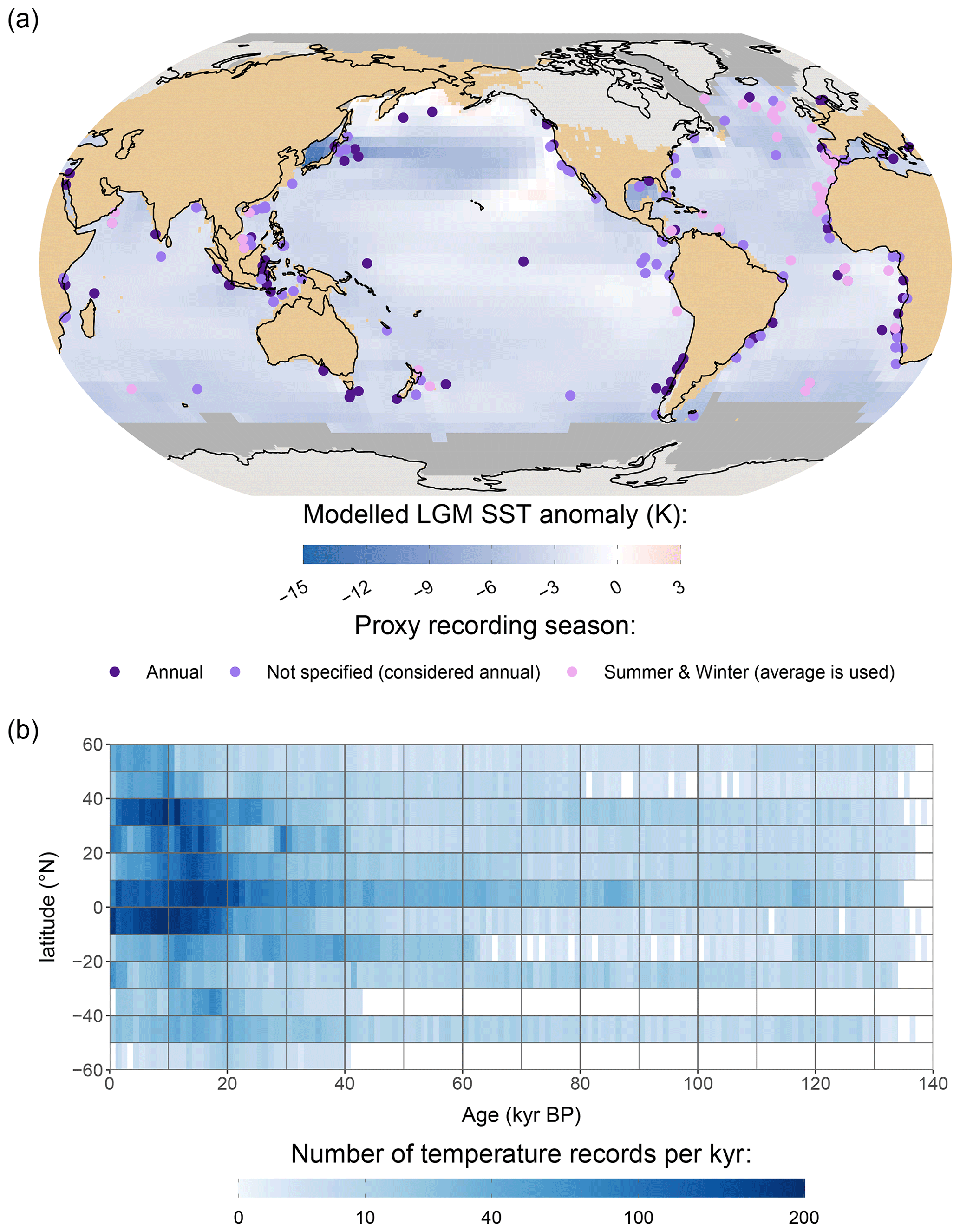
Figure 1 Spatial and temporal distribution of the selected temperature proxy records. Panel (a) shows the locations of inferred sea surface temperature (SST) time series between 60° N and 60° S available in version 2.0 of the PalMod 130k marine palaeoclimate data synthesis and used for this study. Colours indicate whether the recording seasons of the time series are labelled as annual (violet), are not indicated (purple), or whether both summer and winter time series are available (lilac). The background shows, over the ocean, the LGM (19–23 kyr BP) anomaly of SST from MPI-I6G as an example (see Sect. 2.2). Ice-free land (brown) and ice sheets (light grey) are taken from ICE-6G (Argus et al., 2014; Peltier et al., 2015). Darker grey in the ocean corresponds to sea-ice-covered areas in the simulation. Panel (b) represents the latitudinal and temporal distribution of the SST proxy time series from the above panel. The number of proxy data points is given in latitudinal bands of 10° and 1 kyr.

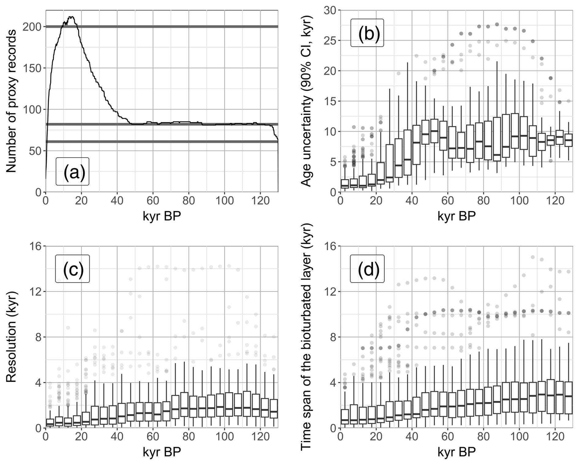
Figure 2 Characteristics of the proxy records in the J20 database. In panel (a), the number of records is computed using the entire time span of the time series. The horizontal grey lines correspond to the values 61, 82, and 200 used in the pseudo-proxy experiments (see Table 2). In panels (b), (c), and (d), the investigated characteristic is averaged over a 5 kyr bin for each time series so that the box plots represent the distribution over the ensemble of records. The bioturbated layer in panel (d) is computed as the bioturbated layer width (fixed at 10 cm) divided by the accumulation rate so that the layer width can be interpreted as a period of time.

2.2 Climate model output

To compute the pseudo-proxy time series used in the PPEs, we use transient simulation outputs from four different climate models: FAMOUS, LOVECLIM, CESM, and MPI-ESM. This multimodel approach is used to test the robustness of the result.

The FAst Met Office and UK Universities Simulator (FAMOUS) is a version of the Hadley Centre Coupled Model version 3 (HadCM3;  Gordon et al., 2000) AOGCM with reduced resolution (Smith et al., 2008). The simulation used here is the version ALL-5G produced in the QUEST project and covers the last 120 kyr (Smith and Gregory, 2012). The simulation is forced with transiently changing orbital parameters (Berger, 1978), greenhouse gas concentrations (Spahni et al., 2005; Lüthi et al., 2008), and Northern Hemisphere ice sheet extents and topographies from the ICE-5G v1.2 dataset (Peltier, 2004).¹ The time-varying external boundary conditions are accelerated by a factor of 10 in the simulation, such that the last 120 kyr are effectively simulated in 12 kyr in the model (Smith and Gregory, 2012).

LOch-Vecode-Ecbilt-CLio-agIsM (LOVECLIM) is an Earth system model of intermediate complexity (Goosse et al., 2010), that is, with coarser spatial resolution and simpler representation of physical processes than in general circulation models. The simulation used here (LOVECLIM 800k; Timmermann and Friedrich, 2016) uses version 1.1 of LOVECLIM (Goosse et al., 2007), with only the atmospheric, oceanic, and vegetation modules activated. Greenhouse gas concentrations are prescribed following the measurements from the EPICA DOME C ice core (Lüthi et al., 2008), and the evolution of ice sheets (surface elevation and albedo, land–sea mask) is prescribed following a simulation with the CLIMBER-2 model (Ganopolski and Calov, 2011). Finally, orbital configurations are derived from Berger (1978). Similarly to FAMOUS, the external forcings are accelerated by a factor of 5.

Several simulations of the last 26 kyr, using MPI-ESM 1.2 (Mauritsen et al., 2019), have been published in Kapsch et al. (2022). We select two simulations from this paper. The first simulation (called GLAC1D-P2 in Kapsch et al. (2022), hereafter MPI-G1D) is forced using the GLAC-1D ice sheet reconstruction (Tarasov et al., 2012; Briggs et al., 2014). By contrast, the second simulation (ICE6G-P2 in Kapsch et al. (2022), hereafter MPI-I6G) uses ICE-6G (Peltier et al., 2015). Forcings are otherwise identical (Köhler et al., 2017, and Berger, 1978, for greenhouse gases and insolation, respectively). These simulations also include meltwater flux forcing from ice sheet melt through a dynamical routing.

Finally, we use a simulation of the last 3 million years (Yun et al., 2023), based on CESM 1.2. (Hurrell et al., 2013). For our period of interest, it uses as boundary conditions an LGM land–sea mask, greenhouse gas concentrations from the EPICA DOME C ice core (Lüthi et al., 2008), orbital configurations from Berger (1978), and the ice sheet elevation and albedo from a CLIMBER-2 simulation (Willeit et al., 2019). The time-varying boundary conditions are accelerated by a factor of 5. Open-access data availability is limited to millennial averages, which restricts the use of this simulation in our analysis.

3 Methods

We first present the GMST reconstruction algorithm, which is an adaptation of S16 (Sect. 3.1). Then, we describe the design of PPEs to evaluate the reconstruction quality (Sect. 3.2).

3.1 Global mean surface temperature reconstruction

3.1.1 The S16 algorithm

The original S16 algorithm reconstructs GMST over the Pleistocene following four main steps.

Firstly, all the irregular raw time series are brought to a common, equidistant (1 kyr) time axis. Then, the time series are smoothed using a Gaussian kernel, which represents the effect of age uncertainty (a constant 10 kyr as the 95 % interval). The algorithm also estimates the signal's standard deviation arising from age, measurement, and calibration uncertainty. The measurement and calibration uncertainty are defined as a standard deviation of 1.5 K, a value similar to other reconstruction studies (Shakun et al., 2012; Tierney et al., 2020). The SST anomalies are finally computed with respect to the late Holocene (0 to 5 kyr BP).

Secondly, the considered domain between 60° S and 60° N is subdivided into latitudinal bands (with nine different configurations), used to cluster the records. The objective is to calculate SST anomalies for each band. Therefore, this latitudinal subdivision is based on the assumption that temperature anomalies are approximately homogeneous within each band (Rohling et al., 2012). This method is a trade-off to still account for the heterogeneity of the record locations, despite the sparsity of the available SST records. At this stage, a Monte Carlo approach is used to propagate the signal uncertainty from each record to the zonal band averages. Specifically, independent realisations of the signal uncertainty are used for each record to compute 1000 zonal band averages, for each of the nine band configurations. Then, n time series are randomly selected from all the time series available (the number of records times the 1000 realisations of the previous sampling), where n is the number of records. That way, the algorithm can evaluate the uncertainty related to the selection of records and, in particular, to their location.

Thirdly, the zonal band averages are aggregated to derive a 60° S to 60° N SST anomaly.

Fourthly, the mean SST anomaly is scaled to a GMST anomaly. Similarly to other studies (Bereiter et al., 2018; Friedrich and Timmermann, 2020), a linear scaling coefficient is used to account for the stronger cooling of polar and terrestrial regions compared to the spatial mean SST change between 60° S and 60° N. The coefficient is derived from PMIP2 and PMIP3 LGM and pre-industrial simulations (Braconnot et al., 2007, 2012). A Monte Carlo approach is again used to quantify the uncertainty: 5000 different realisations of the scaling factor (defined as a Gaussian distribution with a mean of 1.9 and a standard deviation of 0.2) are applied to randomly selected realisations of the mean SST anomaly.

3.1.2 Adaptation of S16 algorithm

We decided to adapt the S16 algorithm to make full use of the J20 dataset (age ensembles, records with no data in the last 5 kyr) and to improve the uncertainty quantification by the algorithm.

Firstly, we apply the measurement and calibration noise before the interpolation of the raw time series. That way, the uncertainty depends on the number of measurements performed: averaged over the same time span, a high-resolution record should have a reduced uncertainty compared to a low-resolution one. We consider 1000 different samples of this noise to quantify the uncertainty.

Secondly, we make use of the age ensembles available for each record in the J20 database: each time series is interpolated using one of the 1000 age ensemble members. A different realisation of the measurement and calibration noise is used for each of these time series. This method lends itself to the Monte Carlo approach used later in the S16 algorithm and avoids any assumption on the distribution of the age uncertainty. We also use a centennial time step for the interpolation so that the higher frequency variability of the reconstructed GMST can be investigated.

Thirdly, 96 records from the J20 database do not cover the reference period 0–5 kyr BP, from which the SST anomaly is computed. Including them increases the number of available records for the period 40–120 kyr BP by 60 %. Therefore, we implement a zonal iterative offsetting procedure. We assume that the SST anomalies are homogeneous enough within each latitudinal band so that the offset needed to compute the SST anomaly of one record can be derived from the others. In each of the zonal bands, the time series are adjusted iteratively, with respect to all previously adjusted time series, according to the following steps:

1. Preliminary step. All records in the considered zonal band are sorted by the age of their most recent data point, starting with the closest to the present.

2. First offsetting. The temperature anomaly of the record including the most recent age is computed with respect to the most recent 5 kyr of that same record.

3. Iterative offsetting. We now consider the interval consisting of the most recent 5 kyr of the next non-adjusted record with the most recent age. We compute the mean of all the already adjusted time series in the zonal band over this interval. The offset of the new record is then calculated such that this mean equals the average temperature anomaly of the new record over the same interval.

Fourthly, all latitudinal bands are averaged using an area-weighted mean, where the weight is proportional to the oceanic surface, instead of the entire surface of the band in S16. For this, we use the ICE-6G reconstruction (Peltier et al., 2015) of the LGM for the entire time period, assuming that changes in oceanic surfaces in each band are small enough compared to other uncertainty sources to be neglected.

Finally, as in S16, the resulting Monte Carlo realisations are used to compute summary statistics of the GMST reconstruction, namely mean and 95 % confidence interval. However, in our case, each GMST time series does not span exactly the same time period because they are based on different sets of age models. Therefore, the statistics are computed only when values from at least half of the realisations are available.

3.2 Pseudo-proxy experiments

We evaluate the algorithm using pseudo-proxy experiments (PPEs). The general design of a PPE is presented in Fig. 3. Pseudo-proxies are artificially generated proxy data created from a reference climate evolution – in our case, temperature outputs from transient simulations. Thus, we apply the GMST reconstruction algorithm to these pseudo-proxies to analyse how well the reference GMST evolution, i.e. the GMST of the transient simulations, is recovered by the reconstruction algorithm. In this idealised setting, influences of individual aspects of the algorithm or characteristics of the data can be studied using sensitivity experiments. In the following, we first describe the strategy to construct pseudo-proxies before presenting the design of the PPEs we perform.

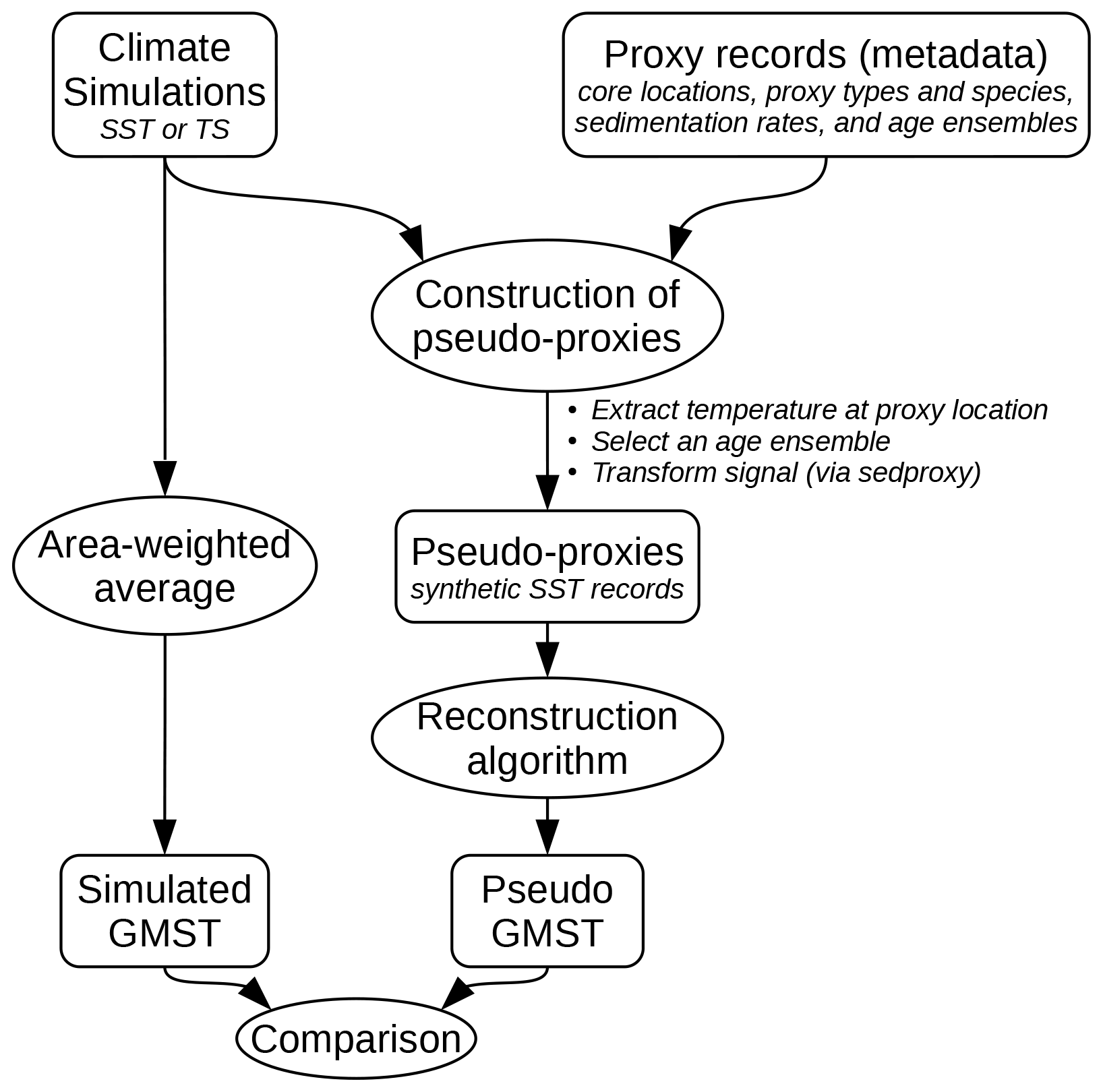
Figure 3 Flowchart summarising the data processing for a pseudo-proxy experiment. Rectangles are for data, while ellipses are for data processing. The metadata proxy records are from the J20 database. The reconstruction algorithm is the modified version of S16. The signal transformation from sedproxy includes habitat preferences, bioturbation, and measurement and calibration noise

3.2.1 Construction of pseudo-proxies with sedproxy

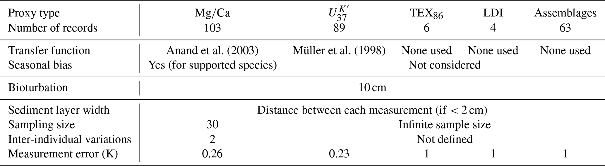
Pseudo-proxies are created by simulating the processes that contribute to the recording of a climate signal in an archive. Here, we use the R package sedproxy to simulate these processes for marine sediment records (Dolman and Laepple, 2018, 2023). More specifically, the package provides a forward model that converts an ocean temperature time series with monthly resolution into pseudo-proxy time series with the desired resolution. Table 1 summarises the processes simulated for each proxy type and the associated metadata. The algorithm implemented in sedproxy consists of four steps.

Firstly, the input temperature data are converted to the relevant proxy unit using well-established calibrations (forward model). This forward model represents the dependency of a process to ocean temperature (the sensor), such as the calcite formation in foraminiferal tests, which uses both Ca or Mg ions, in a proportion depending on the temperature (Nürnberg et al., 1996). This model corresponds to the inverse of the calibration function used to infer temperature from proxy measurements. This step is needed to consider the structure of the calibration error. Note that the calibration for TEX₈₆ and LDI is not yet implemented in sedproxy. Given that it concerns only 10 records, the impact on our analysis should not be significant. In addition, calibration methods used for assemblages in J20 are heterogeneous, and no established forward models, as needed in this first step, exist. Hence, no conversion is performed for these 63 records either. This limits insight into the error structure, but it cannot be overcome with our current framework.

Secondly, for each time point (in fact, sediment depth) for which the proxy record is to be modelled, the algorithm computes monthly weights. These weights represent the chance for the sensor to have recorded the temperature of that specific month and year. The weights combine effects from seasonal preferences of species, bioturbation, and sediment thickness of the sample (for an exhaustive description, see Dolman and Laepple, 2018). In sedproxy, overrepresentation of high-abundance periods, such as particular seasons, is only implemented for $\mathrm{Mg}/\mathrm{Ca}$ ratios, although models for alkenones do exist (Tierney and Tingley, 2018). These preferences are based on the recording species indicated in J20 and computed in sedproxy using the FAME v1.0 model (Roche et al., 2018). For 16 of the records, no seasonal preference is applied, as no growth model is provided for the associated species (namely N. incompta, G. inflata, G. truncatulinoides, P. obliquiloculata, and G. crassaformis). Bioturbation is modelled as a low-pass filter (Berger and Heath, 1968). It supposes a constant bioturbated layer width, which is fixed at 10 cm in our study (default value; see  Boudreau, 1998; Zuhr et al., 2022). While other studies have suggested lower values (Teal et al., 2008; Zhang et al., 2024), we consider this a conservative approach to our analysis. It also requires sedimentation rate as input, which we derive from the depth and mean age available in J20. The impact of the sediment thickness of the sample is also modelled at this stage. In our study, it is computed from the difference between two sample depths but not higher than 2 cm. Finally, for $\mathrm{Mg}/\mathrm{Ca}$ ratios, sedproxy samples 30 pseudo-proxy values whose temporal distribution follows that given by the monthly weights. This sampling corresponds to the number of foraminifera needed to produce a measurement (30 is the default value in Dolman and Laepple, 2018). sedproxy also adds to these values an error corresponding to the inter-individual variability (standard deviation of 2 K;  Dolman and Laepple, 2018) and eventually takes the average over the 30 samples. This sampling process is irrelevant for both $U_{\mathrm{37}}^{K^{\prime }}$ and TEX₈₆: the sample size is considered infinite, and the pseudo-proxy values are based on a weighted mean using the monthly weights. For assemblages, this sampling would be relevant, but what is implemented in sedproxy is too simple to represent it and is dependent on a forward model (see previous paragraph); therefore, it is not considered.

The third stage of the algorithm consists of applying a random Gaussian noise depending on the measurement error. This one is set to 0.26 K and 0.23 K for $\mathrm{Mg}/\mathrm{Ca}$ ratios and $U_{\mathrm{37}}^{K^{\prime }}$, respectively (Dolman and Laepple, 2018). Unfortunately, no standard measurement errors are available for TEX₈₆ and assemblages, so we arbitrarily set it to 1 K. This large uncertainty aims to quantify the impact of not using forward models for the temperature-to-proxy calibration.

The fourth step of the algorithm consists of converting the time series from proxy unit back to temperature. Calibration uncertainty, which arises from using empirical relationships inferred from imperfect data, is only considered at this step. This is done by sampling the calibration parameters using a Gaussian distribution.

In addition to, and before applying, sedproxy, we add a step to account for age uncertainty. Specifically, we randomly select one age member among the 1000 available so that sedproxy computes the pseudo-proxy values at these specific time points. The resulting time series is then associated with all the age ensemble members available.

Finally, the input data for sedproxy correspond to the temperature of the oceanic grid point nearest to the proxy location. For LOVECLIM, MPII6G, and MPIG1D, we use the topmost level of ocean temperature. We use air temperature for FAMOUS and surface temperature for CESM instead, with a screen for land mass and values below −2 °C, so that the seasonality can be investigated.

Anand et al. (2003)Müller et al. (1998)

Table 1 Processes simulated in sedproxy for each type of proxy. The values are those suggested in Dolman and Laepple (2018). The parameter for the bioturbation is the bioturbated layer width.

3.2.2 Specification of the pseudo-proxy experiments

Table 2 Characteristics of the PPEs. The first set is used to analyse the uncertainty sources. The second set, with the addition of “Full PP” and “Measurement noise”, is used to investigate the representation of the time continuum. Apart from “Full PP at random locations”, the number of time series considered depends on the simulation time span: 225 (MPI), 263 (FAMOUS), and 265 (LOVECLIM, CESM). J20 corresponds to the use of metadata from J20. J20* refers to special cases described in the text. Some PPEs are computed several times to form an ensemble. This allows the sampling of measurement noise, random location, or reconstructed age ensemble when applied. The figures where the corresponding PPE is used are indicated in the last column. The results of “Full PP at random locations” are only discussed in the text.

Different sets of PPEs are designed, first to evaluate the performance of the algorithm and then to test the influence of various data properties on the reconstruction. The characteristics of the pseudo-proxies computed for each PPE are summarised in Table 2. In the following, we further describe the method to compute the pseudo-proxies and discuss the rationale of each experiment.

The “Full PP” experiment is used to evaluate the performance of the algorithm under normal conditions. The pseudo-proxies are computed as described in Sect. 3.2.1. The computation of the pseudo-proxies is performed 10 times to test the robustness of our results to the random elements in the methodology (measurement, calibration, and age uncertainty when applying sedproxy). The individual contributions of the five sources of uncertainty quantified by the algorithm are also determined. We indicate in the following in parentheses how each uncertainty quantification is switched off: the measurement and calibration noise (no noise is added), the age model ensemble (only the mean age is considered), the selection of records (all time series are used), the latitudinal band configurations (only the configuration splitting the domain in bands of 20° is considered), and the scaling factor (no uncertainty is applied).

The “Measurement noise” experiment only includes the measurement uncertainty from sedproxy (along with the calibration uncertainty) and its estimate from the algorithm. The experiment is used to compare the representation of measurement noise in the algorithm with the one introduced in the pseudo-proxy and to quantify the effect of the latter on the signal quality. To investigate this effect, we perform 30 iterations of the PPE.

The experiment “SST at proxy locations” is designed to evaluate the ability of the algorithm to recover the 60° S–60° N mean SST signal, given the number and locations of the proxy data. None of the processes modelled by sedproxy are included; that is, the GMST algorithm is directly provided with the modelled SST time series at the grid point nearest to the proxy location.

“Full PP at random locations” corresponds to a series of PPEs investigating the influence of the number of proxy records on the uncertainty. Four numbers are tested: 61 is the number of records selected in S16, 82 is the average number of records during MIS3 to 5 in our dataset (Fig. 2a), 200 is the minimal number of records during the deglaciation, and 400 is an example in the case where a much larger dataset could be obtained. Oceanic locations are randomly generated for each pseudo-proxy. To each of these locations, we assign metadata (proxy type and species) that correspond to a random record in J20 located within 5° of latitude. To construct age models, we start by selecting 100 age ensemble members from each of the 44 (for the MPI simulations) or 24 (for FAMOUS and LOVECLIM) sediment cores that fully span, respectively, the deglaciation (2–25 kyr) and the LGC (5–130 kyr). The age models are then interpolated so that their mean resolution is 100 years. This creates 44 or 24 age ensembles that are randomly assigned to a location. Finally, these metadata are used to compute pseudo-proxy time series with sedproxy. Effects from bioturbation and sediment thickness are removed, as they do not impact the uncertainty estimates of the algorithm. This procedure is iterated 100 times for each number of pseudo-proxy records tested so that an uncertainty range can be drawn from the ensemble.

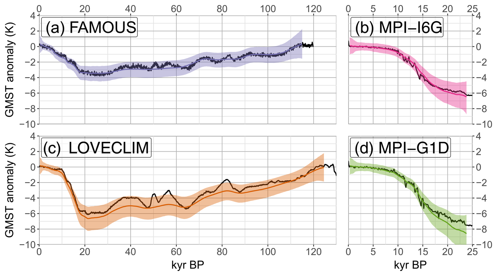
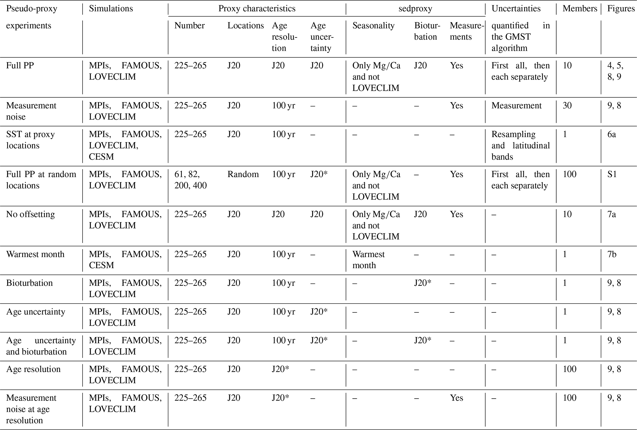
Figure 4 Comparison of the simulated GMST (black lines) and the corresponding reconstructed GMST (coloured line) for each simulation. The reconstructed GMST is based on the pseudo-proxies from the “Full PP” experiment. The shading corresponds to the 90 % confidence interval of the reconstruction. Here, we consider the mean across the 10 computed members. The anomaly is computed with respect to the late Holocene (0 to 5 kyr BP).

The “no-offsetting” experiment is used to evaluate the impact of the offsetting procedure: this one is removed from the algorithm, and the correct temperature anomaly of the simulation at each location is used instead. The experiment is otherwise identical to the “Full PP” experiment. The “warmest-month” experiment is used to estimate an upper bound of seasonality bias on the proxy records. The pseudo-proxies are computed by only considering the warmest month within each year.

The next three experiments evaluate the individual impact on the signal of bioturbation, age uncertainty, and age resolution, respectively, using a simple and idealised setup. In the “bioturbation” experiment, the accumulation rate is identical at each location and is equal to the average across the entire J20 dataset (but still time-dependent; see Figure 2d). Note that we consider bioturbation together with the sediment thickness, as the two are intertwined in sedproxy. For the “Age uncertainty” experiment, we use the same 44 or 24 age ensembles computed for the experiment “Full PP at random locations” to consider age uncertainty independently from other parameters. We consider this selection of age ensembles to closely represent the age uncertainty as a function of time for the entire proxy dataset (as given in Fig. 2b). Finally, for the “Age resolution” experiment, we construct age models for the entire time period which resemble the original distribution of temporal resolutions across time (Fig. 2c). The experiments “Age uncertainty”, “Bioturbation”, and “Measurement noise at age resolution” investigate combined effects.

Finally, note that CESM data have a temporal resolution that is too low to be able to consider the smoothing factors applied by sedproxy and that LOVECLIM data do not enable the investigation of seasonality.

4 Results

The various pseudo-proxy experiments are analysed in this section. We start with the “Full PP” experiment, whose results are presented in Fig. 4. This experiment gives a general overview of the ability of the GMST reconstruction algorithm. In particular, the algorithm successfully reconstructs the orbital timescale variations (>10 kyr) of the four simulations. The mean pseudo-proxy reconstruction, however, presents a strong smoothing of shorter timescales. Finally, the temperature anomaly of the glacial period in the pseudo-proxy reconstructions is, for most simulations, slightly too cold, although the targeted simulated GMST is within the reconstruction uncertainty range. In light of these preliminary results, we arrange the analysis of the results around three main topics, addressed in the following subsections: quantification and origin of the uncertainty, amplitude and timing of orbital timescale variations, and representation of the timescale continuum.

4.1 Quantification and origin of the uncertainty on the GMST

4.1.1 Uncertainty range as estimated by the algorithm

The GMST reconstruction algorithm estimates uncertainties using a Monte Carlo approach. Five different sources of uncertainty are estimated at different stages of the algorithm: measurement and calibration noise, age model uncertainty, selection of records (which we interpret as a location resampling), latitudinal band configurations, and scaling factor. The uncertainty is propagated to the GMST reconstruction by considering an ensemble of realisations.

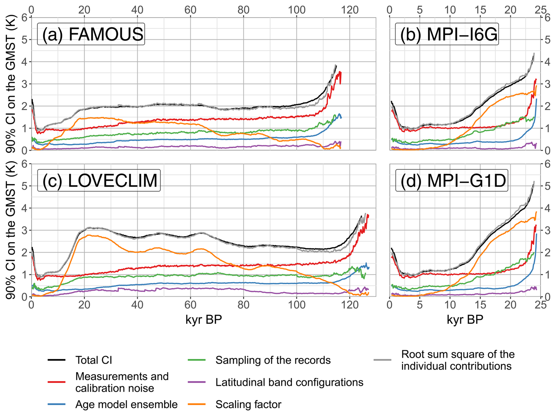
Figure 5 Estimation of various sources of uncertainty for the “Full PP” experiment. The uncertainty is quantified as the width of the 90 % confidence interval (CI) of the reconstructed GMST ensemble. The black lines correspond to the CI in Fig. 4. The coloured lines are the individual contributions of each source of uncertainty quantified in the GMST reconstruction algorithm. Note that we interpret the CI arising from the selection of record as a location resampling. The grey line is the root-sum-square of the individual contribution. It should correspond to the black line if the individual contributions are independent of each other.

The width of the total 90 % confidence interval (CI) is presented in Fig. 5, for the various simulations, alongside an estimation of the individual contributions of the considered uncertainty sources. Note that the uncertainty estimates do not depend on the uncertainty sources accounted for when creating the pseudo-proxies. We first notice a large uncertainty increase at both ends of the time series. The Holocene otherwise has the lowest uncertainty (∼ 1 K for all simulations). The uncertainty is maximum during the LGM (2–4 K). We also find that the root-sum-square of the individual contributions is very close to the total confidence interval. This implies that reducing the uncertainty from the highest sources of uncertainty is the most impactful.

One of the most important contributors to the uncertainty estimate is the scaling factor. By definition, it is proportional to the temperature anomaly and therefore exhibits large fluctuations. It is negligible during the Holocene and the LIG, but it accounts for between 62 % (FAMOUS) and 80 % (LOVECLIM) of the uncertainty estimate during the LGM, depending on how cold the simulated LGM is. On average, the most important contributor to the uncertainty estimate is, however, the measurement and calibration noise, with a CI width mostly between 1 and 1.5 K and an average contribution from 38 % (LOVECLIM) to 50 % (FAMOUS, MPI-I6G). It also increases sharply at both ends of the time series and is the main contributor to the same behaviour in the total CI. The confidence interval of the location resampling and the age model are below 1 and around 0.5 K, respectively (or, in terms of average contribution, around 15 % and 6 % for all simulations). Finally, the configuration of the latitudinal bands has the smallest impact on the uncertainty estimate (below 0.5 K, or 1 %).

Figure 6 Potential reconstruction biases and evaluation of the confidence interval. In panel (a), the 60° S–60° N mean SST (MSST) reconstruction from the experiment “SST at proxy locations” is compared to the simulated MSST. The shaded area is the 90 % CI, only estimating uncertainty from location resampling and the latitudinal band configuration. A properly quantified confidence interval should overlay the 0 line 90 % of the time. In panel (b), we apply the scaling factor with uncertainty to the simulated MSST. We then subtract the GMST from the result. As above, a properly quantified confidence interval should overlay the 0 line 90 % of the time.

4.1.2 Ability of the algorithm to estimate the uncertainty

We further the analysis by investigating whether the GMST reconstruction algorithm correctly estimates the uncertainty sources. We can use the PPEs that only include one uncertainty source and compare them to the estimates from the algorithm. We start with the measurement and calibration noise. By definition, the 90 % CI should have a coverage frequency of the targeted signal of 90 %. However, using the “Measurement noise” experiment, we find that the 90 % coverage frequency is already reached by a CI, smaller than the 90 % CI by a factor of 2 (FAMOUS) to 2.3 (all the others). The overestimation of the CI is not unexpected: the measurement noise introduced in the pseudo-proxies by sedproxy is between 0.23 and 1 K (see Table 1), while the noise introduced in the reconstruction algorithm is 1.5 K. This overestimation is a conservative approach in case the measurement and calibration uncertainty is higher in reality than what is used to compute the pseudo-proxies.

Next, we evaluate the ability of the reconstruction algorithm to estimate the 60° S–60° N mean SST (MSST; before applying the scaling factor) based on the specific set of proxy locations made available in the J20 dataset. To that end, we compare the MSST reconstructed from the “SST at proxy locations” experiment to the simulated MSST (Fig. 6a). We find that the reconstruction for all simulations exhibits a cold bias during the LGM (up to 0.5 K) and most of the glacial period. In addition, location resampling and latitude band configurations, which aim to account for it, are not large enough to cover the bias, yet the pseudo-proxy experiments using random proxy locations can reproduce the simulated MSST (Fig. S1 in the Supplement). Therefore, the bias is caused by the specific set of locations in the J20 dataset: there is an over-representation of regions with strong LGM cooling (e.g. the North Atlantic and the origin of the Kuroshio Extension) compared to regions with weaker to no cooling (e.g. Pacific gyres) in the same latitudinal band (see Fig. 1a, Fig. S3). In addition, how the uncertainty from the location sampling of records is estimated relies on the hypothesis that the temperature anomalies are well distributed, which is not the case, explaining the underestimation of the uncertainty range.

The last uncertainty estimate we evaluate is the scaling factor (Fig. 6b). We find the errors constrained within 1 K. The coverage frequency of the 90 % CI ranges between 46 % (MPI-I6G) and 79 % (LOVECLIM), which denotes a small underestimation. By definition, the uncertainty of the scaling factor is proportional to the temperature anomaly. We suggest that this overly strong constraint leads to an overestimation (underestimation) of the uncertainty for large (small) temperature anomalies. This can be tackled by considering, in addition, an additive error independent of the SST anomaly.

4.1.3 Factors influencing the uncertainty estimates

We continue the analysis by investigating the dependency of the uncertainty estimates. Using the experiment “Full PP at random locations”, we find the number of records considered to strongly impact the uncertainty. Using 61 proxies as a baseline (number of records in S16), we find that 83 records (average number of records between MIS3 to 5) reduce the uncertainty range of the reconstruction by ∼ 15 % (see also Fig. S1). With 200 (as during the deglaciation), the reduction reaches 46 %. In the case where 400 records were available, the reduction would be 62 %. This reduction mostly affects the band configurations and the measurement noise, followed by the location resampling and age uncertainty (in relative values). The proxy number has by definition no effect on the scaling factor.

The variation in the number of records through time in the “Full PP” experiment (Fig. 2a) explains most of the variations in the uncertainties shown in Fig. 5 and, in particular, the increase at both ends of the time series. Note that the number of records considered in the PPE at both ends of the time series is not only related to the number of records available in J20 (see Fig. 2a) but also to the fact that some pseudo-proxy values cannot be computed as age uncertainty spans beyond the time span of the simulations. This is most evident in the MPI simulations (Fig. 5b and d). In addition, measurement noise also depends on the age resolution, as a higher number of measurements reduces the noise introduced in the reconstruction algorithm. The location sampling uncertainty depends on the homogeneity of the temperature anomaly field – that is, to the first order – on the GMST anomaly. Finally, uncertainty due to the age model is dependent on the rate of change of the GMST: abrupt changes such as the deglaciation or the millennial-scale variability exhibited in the MPI simulation or LOVECLIM increase the uncertainty. However, these effects only become noticeable once the number of records is fixed.

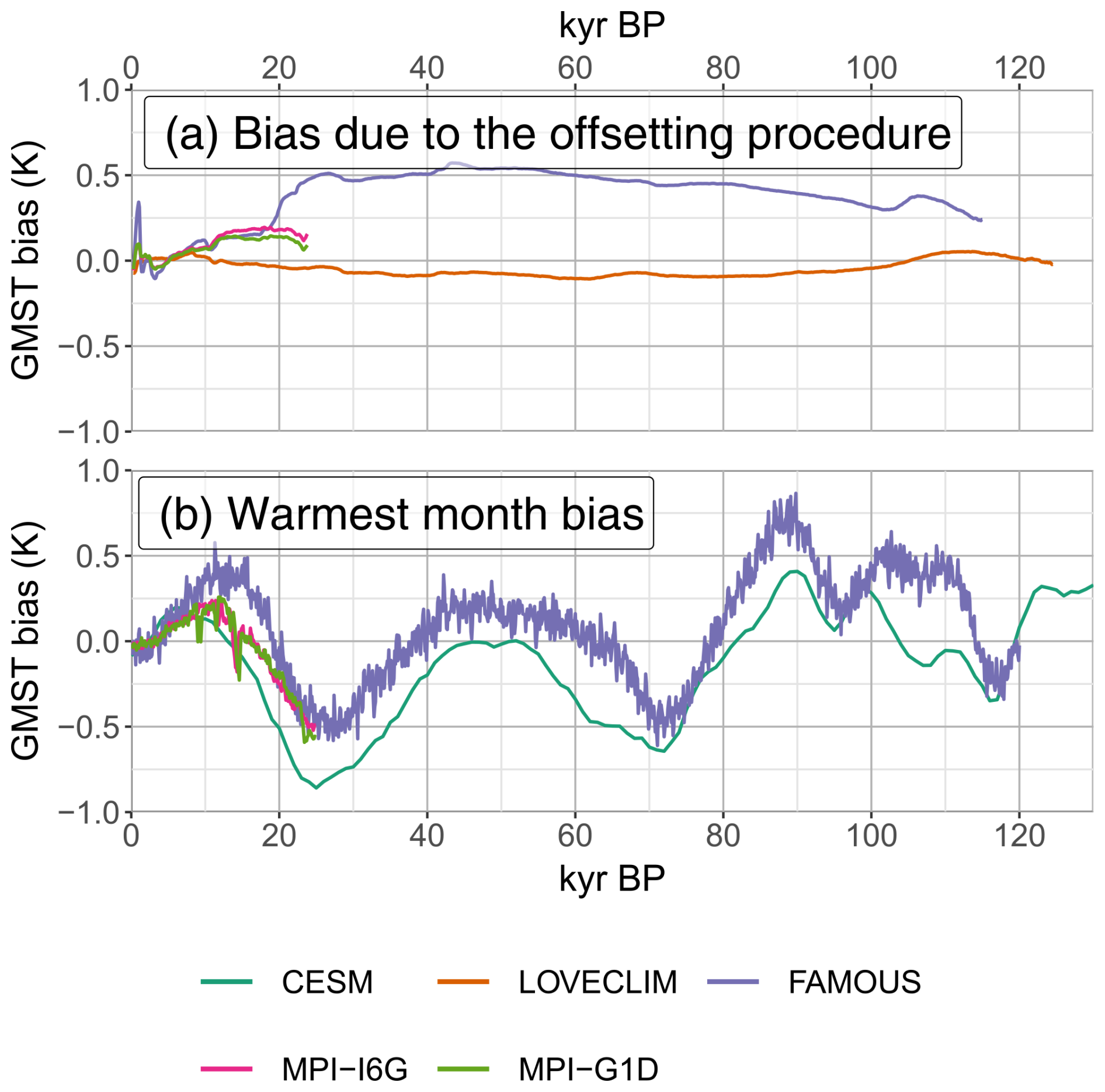
Figure 7 Other potential sources of biases, non-quantified in the uncertainty range. (a) The GMST reconstruction from the “Full PP” experiment is subtracted from the one of the “no-offsetting” experiment. Positive values mean that the offsetting procedure produces a reconstruction that is too warm. (b) The GMST reconstruction from the “SST at proxy locations” experiment is subtracted from the one of the “warmest-month” experiment. Positive values mean that reconstructions based on proxies biased towards the warm season are too warm.

4.1.4 Potential sources of uncertainty non-quantified by the algorithm

Finally, we investigate other sources of uncertainty, which are not or only partly estimated by the reconstruction algorithm. We quantify, in particular, the effect of the offsetting procedure and potential seasonal biases (Fig. 6). The offsetting procedure generates errors generally below 0.2 K on the reconstructed GMST, except for FAMOUS, where it reaches 0.5 K. We suggest this bias is reasonable given the number of records it enables the algorithm to additionally consider (96).

We also estimate an upper bound to the effect of seasonality bias on the pseudo-proxy reconstruction. If all records were not recording the mean annual temperature but that of the warmest month, it would generate biases up to 0.75 K. This bias mostly follows the summer solstice insolation at 65° N: warm during the early Holocene, cold during the LGM and MIS4, and warm again during MIS5. These precession-scale biases can significantly impact the evaluation of this timescale, in particular regarding the LGM cooling, which it could overestimate, or an early Holocene warm period which would only appear for the summer months.

In conclusion, we reckon that the estimation of the uncertainty range by the algorithm is realistic but that the estimations of the individual contributions are biased and should be used with caution. We suggest that the measurement and calibration noise, the set of record locations, and the scaling factor contribute similarly to the uncertainty overall.

4.2 Amplitude and timing of orbital timescale variations

Given the J20 dataset, one of the key characteristics we expect the algorithm to reconstruct accurately is the amplitude and timing of orbital timescale variations of the simulated GMST. While these characteristics can be qualitatively assessed in Fig. 4, we also provide quantitative metrics with uncertainty and robustness (Table 3). Note that we use slightly different definitions for the LGM and the end of the LIG to accommodate the period and behaviour of the simulations (see Table 3 caption).

As already discussed, a cold bias is evident for temperatures of the LGM and the end of LIG in all simulations but FAMOUS, but the true anomalies remain included in the 90 % CIs. This bias is mostly caused by the location bias (see Fig. 6a), while the other factors (offsetting procedure, scaling to GMST, and seasonality) either reduce or amplify it.

Table 3 Quantitative assessment of the reconstruction of the amplitude and timing of orbital timescale variations. We use the GMST reconstructed for the “Full PP” experiment. The LGM temperature anomaly is computed for LOVECLIM and FAMOUS as the coldest 4 kyr later than 40 kyr BP with respect to the last 5 kyr. The same definition is used for LGM occurrence. Due to the difficulty of defining the coldest period in the MPI simulations, we use the average between 19 and 23 kyr BP instead. The deglaciation end is defined as the last time the temperature anomaly reaches 1/10 of the LGM temperature anomaly. Similarly, glacial onset is defined as the first time the temperature anomaly falls below 1/10 of the LGM temperature anomaly. Finally, we also compute a temperature anomaly for the end of the LIG as the average between 119 and 123 kyr for LOVECLIM and between 110 and 114 kyr BP for FAMOUS. “Mean” is the mean value across the reconstruction ensembles. “Robustness” is the range of the mean value for each of the 10 ensembles computed for the experiment; it characterises the robustness of the mean reconstruction to random factors in the proxy data. “90 % CI” is the mean 90 % confidence interval, as calculated by the GMST algorithm, within each reconstruction ensemble. The target is the actual simulated value.

We also investigate the timing of various events: glacial onset, LGM, and deglaciation end. These metrics are only designed to compare the result of the pseudo-proxy reconstruction to the simulations. We find that the reconstructions very closely match the timing of the simulations. We further suggest that the 90 % CI as calculated by the GMST algorithm largely overestimates the uncertainty. While the overestimated measurement noise helps to account for non-quantified sources of temperature bias in the GMST algorithm, it may also lead to an overestimation of the timing uncertainty, where no biases are evident. Interestingly, the PPE including only bioturbation shows a lag of about half the bioturbated layer, which is not evident in the table. This bias is caused by the non-symmetric shape of the function characterising the sediment surface mixing.

Finally, we find our result robust to different realisations of pseudo-proxies. The measure of robustness also describes a limit under which temperature and timing differences depend on the pseudo-proxy realisation: about 0.5 K and from 0.7 kyr in the Holocene to 5 kyr during the LIG. Interestingly, these values are below the uncertainty associated with individual proxy measurements. In addition, we suggest that this measure characterises the uncertainty better than the confidence interval provided by the GMST algorithm, when comparing values to one another.

4.3 Representation of the timescale continuum

As noted in Fig. 4, the algorithm does not reconstruct the high-frequency variability in the simulated GMST. We further investigate this loss of signal using spectral densities and coherence. We focus on the MSST, as the scaling factor does not influence the high-frequency variability. Figure 8 compares the spectrum of variability of the simulated MSST to the one reconstructed in several PPEs. We first focus on the “Full PP” experiment. The individual Monte Carlo realisations of the reconstruction (light-grey lines) appear to overestimate the power spectral density (PSD) for most timescales but the longest ones. In particular, their PSD exhibits a straight slope for the shorter timescales ($\sim -\mathrm{2}$ K²). The overestimated spectrum is mostly related to the large measurement noise introduced in the GMST algorithm. By contrast, the spectrum of the ensemble mean (darker-grey lines) underestimates variability at most timescale, with a steeper slope (between −2.7 K² for FAMOUS and −3.3 K² for the MPI simulations). The PSD is properly represented only for timescales longer than 10 kyr for the entire LGC and longer than 4 kyr for the last 25 kyr (the latter holds regardless of the simulation). None of the pseudo-proxy reconstructions are able to represent all the characteristics of the simulated PSD, such as the high variability at short timescale in FAMOUS or the high variability at millennial timescale in the MPI simulations. The loss of PSD between the ensemble mean and each member's spectrum is due to a lack of coherence between reconstruction members (i.e. loss of signal).

We further investigate the cause of the underestimated variability of the ensemble mean with sensitivity PPEs. We identify four potential causes: the bioturbation, which smooths the local SST time series; the age uncertainty, which reduces the coherence between the local SST time series; the age resolution, which permits resolving the shortest timescale; and the measurement and calibration noise in sedproxy, which adds non-climatic variability (see coloured lines in Fig. 8). The PSD from the “Measurement noise” experiment (yellow) is the closest to the simulated one with just slight overestimation but loses the simulated PSD characteristics below 1 kyr. In this PPE, the noise is injected at the centennial scale, resulting in increased variability at this timescale and upward propagation. Over the LGC, none of the other PPEs are able to represent the simulated spectrum below 10 kyr, with the strongest loss in PSD due to age uncertainty (blue). For the last 25 kyr, the PPEs are still able to reproduce the large multi-millennial variability, which is only lost by the joint consideration of bioturbation and age uncertainty (purple).

The loss of signal at specific timescales can be further characterised using coherence. Coherence, or the squared coherency spectrum, is a statistical method to analyse the dependency between two time series through the timescales (Von Storch and Zwiers, 1999). It can be seen as a timescale-dependent squared correlation. A coherence of 0 implies that the two time series vary independently at this timescale. A coherence of 1 means that the time series vary synchronously, although a lag can exist. The coherence also does not characterise the amplitude of the variation, which we have already investigated with the spectral densities. Figure 9 presents the coherence between the simulation and reconstructed MSST from the same PPEs as in Fig. 8. For the “Full PP” experiment, coherence is very high (>0.9) for the longest timescales in all simulations. However, the coherence decreases sharply for timescales shorter than 15 kyr for the LGC simulations (FAMOUS and LOVECLIM), which corresponds to the start of the PSD loss in Fig.  8a and c. The drop happens at shorter timescales (below 4 kyr) for the last 25 kyr, again corresponding to the timescale from which the PSD loss starts. A similar timescale has been found for the Holocene (Dolman et al., 2021).

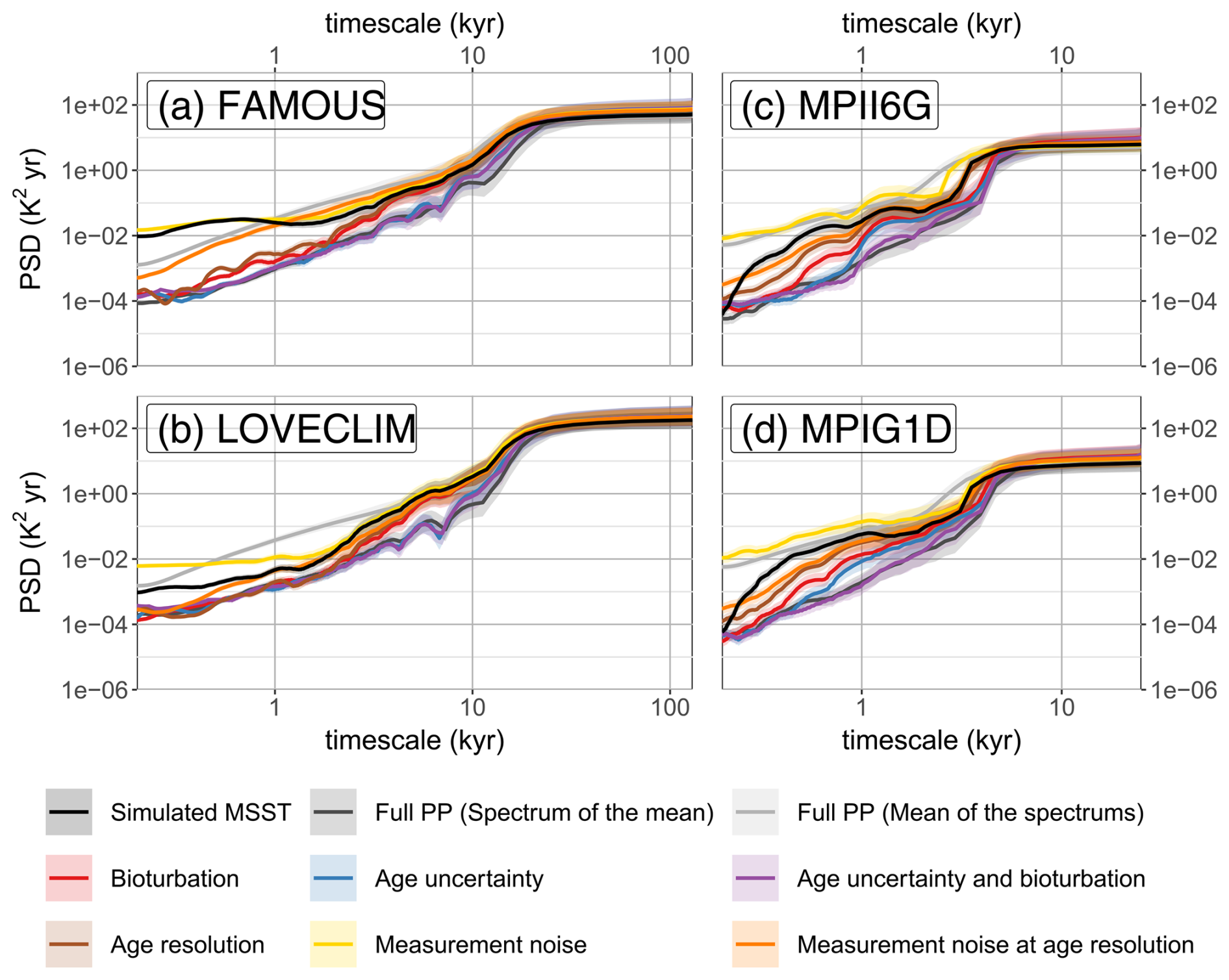
Figure 8 Loss or gain of variability at specific timescales between reconstructed and simulated MSST. The black line is the power spectral density (PSD) of the simulated MSST. The other lines correspond to various PPEs defined in Table 2. For the “Full PP” experiment, we consider both the PSD of the ensemble mean and the PSD of each ensemble member. Only the ensemble mean is considered for the other PPEs. Finally, the shading corresponds to the confidence interval at level 0.05 of the PSD estimates.

Figure 9 Disentangling the origin of the loss of signal at high frequencies. The loss of signal is quantified by the coherence between the simulated and reconstructed MSST for various PPEs. For the latter, we use the ensemble mean. The thicker lines correspond to significant values at level 0.05. Specifically, they are values above the 95th percentile of the coherences between the simulated MSST and randomly phase-shifted time series of the same characteristics.

We further the analysis with the sensitivity PPEs. We find the age uncertainty (blue) to be the main cause of the loss of coherence on the LGC. For the last 25 kyr, bioturbation also plays an important role, but neither can individually explain the coherence loss exhibited by the “Full PP” experiment. In addition, using a smaller bioturbation depth further limits the influence of bioturbation (Fig. S2). Measurement noise (yellow) and age resolution (brown) have the smallest impact on the coherence for either the LGC or the last 25 kyr. However, the measurement noise is in reality linked to the age resolution. The PPE considering both (orange line) exhibits a coherence loss at a timescale close to the age uncertainty and bioturbation, suggesting it also has a key role for the last 25 kyr. Note that, for the number of records considered, the set of record locations does not impact the coherence significantly. Simulated GMST and MSST are also significantly coherent at all timescales (Fig. S5).

Our results show that the difference in results between the LGC and the last 25 kyr is directly related to the dataset characteristics (Fig.  2b–d). In the last 25 kyr, the average 90 % CI of the age uncertainty and the average bioturbated layer have similar values, corresponding to the timescale when coherence is lost. The age uncertainty, resolution, and bioturbated layer increase beyond this time period, but the increase in age uncertainty is the most important. This one reaches ∼ 10 kyr beyond 40 kyr BP, again similar to the timescale when coherence drops.

5 Discussion

The results from the previous section allow us to discuss the performance of the reconstruction algorithm applied to the J20 dataset (Sect. 5.1). Nevertheless, future avenues for these pseudo-proxy analyses are possible (Sect. 5.2). We also discuss which limiting factors from either the algorithm (Sect. 5.3) or the dataset (Sect. 5.4) should be addressed in priority to improve the GMST reconstruction quality.

5.1 Quality of the reconstruction

According to our analysis of the PPEs, the timing of GMST variations can be reconstructed for timescales longer than 4 kyr and a timing uncertainty of ±0.5 to 1 kyr for the last 25 kyr. Beyond 40 kyr BP, only timescales longer than 15 kyr can be reconstructed, with an uncertainty of up to ±3 kyr. This precision of the reconstruction, and its variation through time, is directly related to the underlying dataset characteristics. The reconstruction of shorter timescales beyond 40 kyr BP is limited by the age uncertainty of the records. For the last 25 kyr, the limitation originates from a combination of age uncertainty, bioturbation, and measurement and calibration noise.

Most reconstructed pseudo-proxy GMSTs also exhibit a cold bias of up to 1 K during the glacial period, which we attribute to the specific set of record locations in J20. Uncertainty on the temperature anomaly is otherwise strongly dependent on the number of proxy records and the scaling factor. The GMST algorithm estimates the uncertainty range (90 % CI) from less than 1 K during the Holocene to up to 3 K for a cooling of 6 K during the LGM. Our results suggest, however, that the Holocene uncertainty is overestimated because of an overestimated measurement noise uncertainty. Similarly, the uncertainty for large temperature anomalies is also likely overestimated due to the definition of the scaling factor uncertainty. For the LIG, overestimated measurement noise and underestimated scaling uncertainty seem to cancel each other out and lead to reasonable values. These overestimations nevertheless help to account for uncertainty sources not properly accounted for, such as locations or potential seasonality bias. In particular, an underestimation of the seasonality bias could lead to a deterioration of the performance, both in terms of amplitude and timing of variations, especially for the period between the LGM and the early Holocene, where uncertainty is otherwise the lowest.

The analysis of the uncertainty of the timing and amplitude of variations shows that there exists a trade-off between including many records, which helps to reduce the biases and uncertainty on the amplitude, and including only the records of the highest quality (low age uncertainty, high accumulation rate, high resolution), which help better resolve the shorter timescale variability. While a finer selection of records could balance the two, we also suggest that the algorithm could handle records of different characteristics better (see Sect. 5.3).

These results are robust across the set of simulations, and we assume them to hold for the real-world reconstruction. In addition, while these results are specific to the adapted S16 algorithm applied to J20, we expect that the general concepts discussed here hold for any aggregation algorithm and dataset. In particular, the algorithm could be used for regional reconstructions (as done in  Clark et al., 2024), as long as a sufficiently high number of records is considered. We suggest, for example, that the accurate reconstruction of the timing of orbital timescale variations (>10 kyr) offers a good opportunity to investigate the synchronicity of regional temperature anomalies and forcings.

5.2 Advances in pseudo-proxy experiments

Our results rely on advances in pseudo-proxy experiments, which were enabled by the availability of proxy system models and climate simulation output.

5.2.1 Model data

In addition to the proper availability of simulated climate fields for the production of PPE, the PPE results can only be transferred to real proxy data if these fields are realistic enough. The recent advances in computing capacities, modelling, and our understanding of climate drivers have enabled the production of more realistic climate simulations over longer periods of time (Ivanovic et al., 2016), yet the PPEs we conduct require data only available for a handful of simulations. However, a multi-model framework for PPEs is key to assessing the robustness of our results.

One of the requirements is, of course, the simulated time period, which needs to cover more than the period of interest, to take into account the age uncertainty of the records. For example, properly investigating the LIG requires data from the penultimate deglaciation. Another requirement is that these simulations must include transient forcings so that realistic variations in the GMST can be produced at sufficiently high resolution. In particular, a centennial or lower resolution is needed here to resolve the effect of bioturbation. The addition of other forcings, such as meltwater, in the MPI simulations also increases the degree of realism of the simulated GMST (Weitzel et al., 2024). These additions make more refined analyses of the results possible, which can more easily be transferred to real proxy data. For instance, we can assess that the GMST algorithm is not able to reconstruct the effect of meltwater forcing, such as the abrupt events during the deglaciation.

Finally, the spatiotemporal variability in the simulated climate fields affects our results. For example, the amplitude of the temperature bias due to the proxy locations directly depends on the spatial pattern of the simulated temperature field. Differences between the simulations lead to differences in the estimation of the bias in the PPE reconstruction (see Fig. 6a). Therefore, despite some agreements between simulations on the sign and amplitude of the bias, proper quantification of this bias for real-world reconstructions would first require an evaluation of the degree of realism of the spatiotemporal patterns. In support of this, the temperature field of simulations is known to be more homogeneous at the regional scale compared to proxy records (Jonkers et al., 2023). This has been demonstrated for the multidecadal to multimillennial scale (Laepple et al., 2023; Weitzel et al., 2024). For the orbital timescale (>10 kyr), Paul et al. (2021) suggested that upwelling regions, where many records come from, can have a different variability while being too small to be properly resolved by the models considered here. The use of fields that are too homogeneous can lead to an underestimation of location biases on the reconstructed temperature and overconfidence in the algorithm.

5.2.2 Proxy system models

In PPEs, proxy system models are used to produce pseudo-proxy values that are as realistic as possible. However, proxy system models only represent our current understanding of the proxy system, which limits the extrapolation of our results to the real-world reconstruction. However, the use of sedproxy presents the advantage, compared to more conceptual approaches (e.g. Wang et al., 2014; Jaume-Santero et al., 2020; Nilsen et al., 2021; Weitzel et al., 2024), to model specific processes, such as the measurement and calibration noise and bioturbation, as a function of a record's metadata. Sensitivity PPEs can therefore be computed to evaluate the impact of these processes.

However, our results are also limited by the proxy system model used. For example, the impact of the processes occurring during the sensor stage for TEX₈₆, LDI, or assemblages has only been crudely accounted for within a generic measurement error. We therefore did not investigate in depth the influence of the proxy types on the reconstruction. While increased uncertainty from the measurement or the calibration will reduce the ability of the reconstruction to resolve the shorter timescale, other biases affecting the longer timescale would require a more thorough analysis. These potential biases include, for example, the effect of any variables other than the SST, such as depth, salinity, or seasonality, on the temperature signal recorded (Telford et al., 2013; Timmermann et al., 2014; Ho and Laepple, 2015; Jonkers and Kučera, 2017). The seasonality bias is considered for most species recording $\mathrm{Mg}/\mathrm{Ca}$ ratios in sedproxy but assumed negligible for the other proxy types. For this reason, we design a PPE to estimate an upper bound of the effect of seasonality, where all proxies record the warmest month of the year. This warm season bias has, for example, been one of the main hypothesised reasons for the model–data discrepancies during the early Holocene (Liu et al., 2014; Marsicek et al., 2018; Bova et al., 2021), although there is also evidence for cold-season bias for other periods and species (Steinke et al., 2008; Timmermann et al., 2014).

5.3 Improvement of the algorithm

One of the primary objectives of this paper is to provide a framework to evaluate the performance of GMST reconstruction algorithms. We focus on an adaptation of S16 as an example. The adaptations are minor and only required to improve the use of the J20 dataset and the characterisation of the algorithm's performance (see Sect. 3.1.2). However, our evaluation makes evident avenues of improvement for the algorithm which we discuss here.

We have already discussed how the algorithm is sensitive to the spatial distribution of proxy records. This sensitivity relates to the assumption that temperature anomalies are similar within a latitudinal band. Both the simulations used here and other proxy analyses show that this is not the case (e.g. Judd et al., 2020; Tierney et al., 2020; Paul et al., 2021). Some studies have used more complex methods and relied on either present SST observations (e.g. Paul et al., 2021) or climate simulations (e.g. Osman et al., 2021; Annan et al., 2022). These methods, however, rely on the assumption that the spatial covariance of the present day does not change through time or that the spatial covariance of the simulated SST is similar to the reality. The design of another aggregating method could help to reduce the influence of areas with a large density of records, without relying on external datasets.

Our refined algorithm relies on the stacking of proxy records to increase the signal-to-noise ratio. However, records are stacked together, regardless of their quality (age uncertainty, accumulation rate, resolution). This stacking method leads to a trade-off between data quality, which improves the reconstruction of the shorter timescales, and a high number of records, which reduces the overall uncertainty (see Sect. 5.1). A new stacking method could be researched to limit the impact of this trade-off by, for example, taking into account the timescale resolved by each record.

Finally, the scaling of the MSST to the GMST was introduced by S16 due to the limited availability of reliable local temperature reconstruction over land and ice-covered areas for the investigated time period. Similarly, Clark et al. (2024) use a scaling factor, although with a different definition. This scaling is in both cases a critical source of uncertainty, especially concerning the amount of glacial cooling or LIG temperature anomaly. This directly affects our ability to constrain Earth system sensitivity or the global response to climate forcings. The transient simulations used here show that the variation in GMST and MSST is not completely collinear (Fig. S4). This behaviour suggests going beyond the simple LGM-to-PI ratio used to compute the scaling factor in S16 or even the one-to-one match between MSST and GMST supposed in Clark et al. (2024). Despite their scarcity, the use of terrestrial proxies for temperature could still help to better characterise the scaling, yet large areas lack proxy information, particularly over sea ice and ice sheets that have melted. Physics-based constraints remain needed for these areas.

5.4 Limiting factors from the dataset and future developments

Expanding the dataset with new records, in particular for the periods and areas where fewer records are available, will evidently improve the reconstruction. Nevertheless, spatiotemporal inhomogeneity will always remain due to geological constraints. Other avenues can improve the quality of and the confidence in the reconstruction from the perspective of the proxy dataset. Firstly, the age uncertainty is the limiting factor preventing the reconstruction of a multi-millennial timescale beyond 30 kyr BP, and better characterisation of and constraints on age uncertainty are required. Progress has been made, for example, using visual matching and quantifying the associated uncertainty or considering the impact of bioturbation on age model (e.g. Waelbroeck et al., 2019; Lougheed, 2022; Peeters et al., 2023). In addition to improving the confidence in the absolute age, information on the relative age between records can also be provided, if properly accounted for by the reconstruction algorithm.

Secondly, measurement and calibration noise and bioturbation are other sources of loss of signal on short timescales, particularly in the last 30 kyr. Here, we suggest better quantifying these uncertainties for each record so that the algorithm can sort the records depending on the timescale they can resolve. In particular, bioturbation depth could be quantified for each record, and measurement uncertainty could depend on the number of replications or sample size for each data point.

Finally, we find that potential seasonality bias can significantly decrease the accuracy of the reconstruction. For many of the records available, it is unclear whether the reconstructed temperature suffers from a seasonal bias. Corrections from seasonally biased records have been suggested (e.g. Bova et al., 2021), but they rely on assumptions that must be verified beforehand (Laepple et al., 2022).

6 Conclusions

In this study, we design a framework for the evaluation of algorithms reconstructing spatial mean temperatures. Our framework relies on recent advances in pseudo-proxy experiments, which include the availability of realistic proxy system models and long transient climate simulations. We apply the framework to an adapted version of the GMST reconstruction algorithm used in S16 and the synthesis of marine proxy records for temperatures of the LGC from J20. The quantitative results presented here can serve as a basis for future evaluations of LGC reconstructions, while the framework can be applied to other aggregation-based reconstruction algorithms and other datasets.

Our results are based on PPEs computed from an ensemble of four transient simulations of the LGC or the last 25 kyr. We find that the pseudo-proxy reconstructions based on the S16 algorithm and the J20 dataset perform differently over time. For the last 25 kyr, the temperature variations and their timing are accurately reconstructed for timescales of at least 4 kyr. Sensitivity PPEs show that age uncertainty, bioturbation, and measurement noise smooth the reconstruction, leading to a loss of signal below this timescale. Uncertainties remain large on the amplitude of temperature variations, even for longer timescales, although we find the algorithm to overestimate it. The reconstructions exhibit, in particular, a cold bias for most model simulations, which is related to the non-uniform distribution of record locations. Other sources of uncertainty include the scaling of the mean SST to the GMST, the measurement and calibration noise, and a potential seasonal bias. The number of records plays a critical role in reducing all uncertainty sources but that of the scaling. The decreasing proxy number and increasing uncertainty of the scaling are the two main factors explaining the increased uncertainty from the Holocene to the LGM. Beyond 40 kyr BP, only timescales longer than 15 kyr can be reconstructed, due to a sharp rise in age uncertainty. We assume these results to hold for real-world reconstructions of the LGC.

Our results also show the existence of a trade-off between the inclusion of many records, which overall reduces the uncertainty, and of only the highest-quality records (low age uncertainty, high accumulation rate, high resolution), which improves the reconstruction of the short timescale. The reconstruction could be improved by a better filtering of the input record data or by a better handling of the varying record quality by the algorithm. We also suggest other avenues of improvement for the algorithm to better handle the spatial aggregation and the scaling to GMST. From the proxy record perspective, reducing the age uncertainty is the most critical challenge to tackle.