Using a multi-layer snow model for transient paleo-studies: surface mass balance evolution during the Last Interglacial

During the Quaternary, ice sheets experienced several retreat–advance cycles, strongly influencing climate patterns. In order to properly simulate these phenomena, it is preferable to use physics-based models instead of parameterizations to estimate the surface mass balance (SMB), which strongly influences the evolution of the ice sheet. To further investigate the potential of these SMB models, this work evaluates the BErgen Snow SImulator (BESSI), a multi-layer snow model with high computational efficiency, as an alternative to providing the SMB for the Earth system model iLOVECLIM for multi-millennial simulations as in paleo-studies. We compare the behaviors of BESSI and insolation temperature melt (ITM), an existing SMB scheme of iLOVECLIM during the Last Interglacial (LIG). Firstly, we validate the two SMB models using the regional climate model Modèle Atmosphérique Régional (MAR) as forcing and reference for the present-day climate over the Greenland and Antarctic ice sheets. The evolution of the SMB over the LIG (130–116 ka) is computed by forcing BESSI and ITM with transient climate forcing obtained from iLOVECLIM for both ice sheets. For present-day climate conditions, both BESSI and ITM exhibit good performance compared to MAR despite a much simpler model setup. While BESSI performs well for both Antarctica and Greenland for the same set of parameters, the ITM parameters need to be adapted specifically for each ice sheet. This suggests that the physics embedded in BESSI allows better capture of SMB changes across varying climate conditions, while ITM displays a much stronger sensitivity to its tunable parameters. The findings suggest that BESSI can provide more reliable SMB estimations for the iLOVECLIM framework to improve the model simulations of the ice sheet evolution and interactions with climate for multi-millennial simulations.

1 Introduction

The Quaternary (since 2.6 Ma) has experienced several glacial–interglacial cycles. These episodic periods influenced the whole Earth system, with climate shifting periodically from cold to warm phases and repeated retreat–advance cycles of the ice sheets and glaciers. Ice sheets and their interactions with climate strongly influence phenomena such as sea level evolution (Dutton et al., 2015; Spratt and Lisiecki, 2016; Turney et al., 2020) and changes in the atmospheric circulation (Ullman et al., 2014; Liakka et al., 2016). Ice sheets gain mass through surface accumulation (snow and rain) and internal accumulation (refreezing). In contrast, they lose mass due to melting and sublimation/evaporation processes on the surface or through iceberg calving and sub-shelf melting. The difference between mass gains and losses at the surface is called the surface mass balance (SMB), which plays a significant role in the build-up or disappearance of the ice sheets. Studies of ice sheet evolution through past events unravel the dynamics of glaciation and deglaciation, improving trajectories of ice sheets in the past and confidence in future projections.

Investigating ice sheets and climate feedbacks in such long-timescale periods requires a tool that can simulate the interactions between the main components of the Earth system at a reasonable computational cost. In this context, Earth system models of intermediate complexity (EMICs) are of interest, as they have much lower computational costs compared to state-of-the-art general circulation models (GCMs) while still being able to simulate most of the important processes thanks to their low resolution and simplifications (Claussen et al., 2002; Eby et al., 2013). However, these simplifications result in some drawbacks, particularly in reproducing the evolution of ice sheets. Because of their coarse resolution, EMICs fail to capture the narrow ablation zones in the ice sheets' margin, leading to improper runoff estimation (Ettema et al., 2009; Noël et al., 2019). To mitigate this problem, the output of the atmospheric part can be bilinearly interpolated (Gregory et al., 2012) or downscaled (Quiquet et al., 2021) to provide finer-resolution input to the ice sheet model in the EMIC framework.

Another problem is the missing physical snow models within the EMIC framework to simulate the energy and mass transfer between the surface and the atmosphere (Lenaerts et al., 2019). In general, EMICs mostly utilize simple parameterizations, such as positive degree-day (PDD) (Reeh, 1991) or the insolation temperature melt (ITM) equation (Van Den Berg et al., 2008), due to their simplicity and low computational cost (Born and Nisancioglu, 2012; Stone et al., 2013; Robinson and Goelzer, 2014; Goelzer et al., 2016b; Quiquet et al., 2021). However, as these schemes depend on locally calibrated parameters, their reliability is questioned when climate conditions change or when available data for calibration are limited, particularly in paleo-studies. Bauer and Ganopolski (2017) report a failure of PDD in providing proper SMB values for the last glacial cycle study, which resulted from the albedo feedback being absent in the simulation. This poses a need to include a more physical snow model in such long-term climate simulations. The first option is to use dedicated snowpack models coupled to regional climate models (RCMs), which have abilities to simulate not only the key physical processes of the SMB (melt, sublimation, and snow drifting) but also snow properties such as densities and metamorphism (Fettweis et al., 2017; Noël et al., 2018; Agosta et al., 2019; van Dalum et al., 2022). However, due to their complexity and computational cost, they are not suitable for long-term transient simulations and large study areas. As a compromise between parameterizations and SMB models, intermediate-complexity energy balance models are promising SMB schemes for EMICs to run long simulations of ice sheet studies (Calov et al., 2005; Willeit et al., 2024). These models have the appropriate level of simplicity in their structure and high computational efficiency, such as Born et al. (2019).

To answer the question of whether a physics-based scheme is a better choice for the representation of the SMB on a paleo-timescale, this work evaluates the differences in the behaviors of the simple SMB scheme in iLOVECLIM and a physical-based surface energy balance model, the Bergen Snow SImulator (BESSI) (Born et al., 2019), in a paleo-study. Thanks to its high computational efficiency, iLOVECLIM has been used to carry out many paleoclimate studies ranging from ice sheet–climate interactions during the last deglaciation (Roche et al., 2014a; Quiquet et al., 2021; Bouttes et al., 2023) and Heinrich events (Roche et al., 2014b) to ocean circulation (Lhardy et al., 2021a) and carbon cycle changes between glacial–interglacial states (Bouttes et al., 2018; Lhardy et al., 2021b). BESSI is a surface energy and mass balance model designed for Earth system models of intermediate complexity. The snow model has been used to study the surface mass balance of the Greenland Ice Sheet during different periods (Zolles and Born, 2021; Holube et al., 2022; Zolles and Born, 2024) and proved to have good performance compared to other more complex models (Fettweis et al., 2020). In this work, we evaluate the performance of the updated version of BESSI since Zolles and Born (2021) and ITM: the current SMB scheme of iLOVECLIM for present-day climate using the regional climate model Modèle Atmosphérique Régional (MAR) as forcing and benchmark in the Greenland and Antarctic ice sheets (GrIS and AIS, respectively). By doing this, we assess the models' behaviors under different climate conditions. In the second part, we assess the impact of using iLOVECLIM as the climate forcing on the SMB simulation of BESSI and ITM. Next, we compare the SMB evolution simulated by the two SMB models during the most recent interglacial period, the Last Interglacial (LIG; (130–116 ka), which corresponds to Marine Isotope Stage (MIS) 5e. During this period, due to the change in the orbital configuration of the Earth, increasing summer insolation in the high-latitude regions of the Northern Hemisphere leads to warmer conditions in polar regions (Capron et al., 2014). The estimation of the global mean temperature change during the LIG with respect to the pre-industrial (PI) ranges from almost no change (Capron et al., 2014; Hoffman et al., 2017; Otto-Bliesner et al., 2021) to a 1–2 °C warming (Turney and Jones, 2010; McKay et al., 2011; Fischer et al., 2018). A warming in the high-latitude regions is nonetheless reported by both proxy data and model outputs. In addition, the sea level is reported to be at least 1.2 m higher during the LIG (Dutton and Lambeck, 2012; Dutton et al., 2015; Dyer et al., 2021). Hence, the LIG provides documented records and insights into the behaviors of different Earth system components under warm climates to benchmark models and study the dynamics behind the phenomena (Fischer et al., 2018). This period has been well studied for various aims, such as reconstructing temperature (Lunt et al., 2013; Landais et al., 2016; Obreht et al., 2022) and sea level (Kopp et al., 2013; Dutton et al., 2015) and investigating climate and ice sheet interactions (Bradley et al., 2013; Goelzer et al., 2016a; Sutter et al., 2016). Applying BESSI for the LIG has been done before in the work of Plach et al. (2018) for the Greenland Ice Sheet only by using climate forcings from MAR with equilibrium runs of some LIG time slices: 130, 125, 120, and 115 ka. In our work, as iLOVECLIM is much more computationally inexpensive compared to MAR, we can obtain transient climate forcings for BESSI and ITM to simulate the evolution of the SMB throughout the whole LIG for both the GrIS and the AIS. We select the LIG to investigate the abilities of BESSI and ITM in simulating the evolution of the SMB under different boundary conditions (deglaciation and glacial inception). From this, we can thoroughly investigate the effects of using a more physics-based model in simulating the SMB for an intermediate-complexity Earth model.

Section 2 provides background information about the models and the climate forcings, together with the design of the experiments. The results are presented in Sect. 3, followed by a discussion about the models' behaviors and the climate forcings in Sect. 4. Finally, a summary of the work is in Sect. 5.

2 Methods

2.1 Model description

2.1.1 BESSI

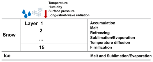
The BErgen Snow SImulator (BESSI) is a multi-layer snow model simulating the surface energy and mass balance with high computational efficiency, designed to be coupled with low-resolution Earth system models (Born et al., 2019). The model, which in its current configuration uses 15 vertical snow layers, requires near-surface air temperature, total precipitation, humidity, surface pressure, and downward long-/shortwave radiation as input. BESSI runs at a daily time step and simulates albedo, which decays exponentially after the latest snowfall event. Based on the energy transfer between the surface and the air, the model simulates important processes of surface mass balance, such as melt, refreezing, runoff, and sublimation/evaporation, which results in the changing mass of the snow column. Among the snow layers, heat diffusion and mass compaction are also simulated (Fig. 1). Compared to the version in  Zolles and Born (2021), in this work, BESSI acquires the incoming longwave radiation flux from the input instead of using parameterization. A detailed description of surface energy and mass balance processes is presented in Appendix A.

Figure 1 Sketch of the BESSI model with required inputs and simulated processes.

2.1.2 iLOVECLIM

The Earth system model of intermediate complexity iLOVECLIM (version 1.1) is a code fork of the LOVECLIM 1.2 model originated from Goosse et al. (2010). The key components of the model include the modules ECBILT for the atmosphere, CLIO for the ocean, and VECODE for the vegetation. ECBILT is a quasi-geostrophic atmospheric model that runs on a T21 spectral grid (Opsteegh et al., 1998). Meanwhile, CLIO is a 3D free-surface ocean general circulation model coupled to a thermodynamic sea ice model and discretized on a 3° × 3° spherical grid (Goosse and Fichefet, 1999). VECODE is a dynamical vegetation model that allocates carbon and simulates land cover and tree fraction on the same grid as the atmospheric model (Brovkin et al., 1997). iLOVECLIM runs with a 360 d calendar.

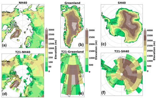
Figure 2 Topography of iLOVECLIM for different resolutions: (a) NH40, (b) NH40 zoomed in on Greenland with the red contour indicating the present-day ice sheet extent, (c) SH40, (d) T21 with a similar projection to NH40, (e) similar to panel (d) but zoomed in on Greenland, and (f) T21 with a similar projection to SH40.

Climate forcings for BESSI are obtained from the online downscaling module within the iLOVECLIM framework, which recomputes the surface energy budget and total precipitation on a subgrid resolution for the ice sheet areas (Quiquet et al., 2018). In this work, we run the downscaling for two polar regions to obtain near-surface air temperature, total precipitation, and humidity on a 40 km × 40 km Cartesian grid (referred to as NH40 and SH40 for the North Pole and the South Pole, respectively) (Fig. 2a–c). To obtain other input variables for BESSI, long-/shortwave radiation and surface pressure are bilinearly interpolated from the native T21 grid (Fig. 2d–f) to the NH40/SH40 grid.

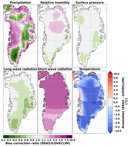
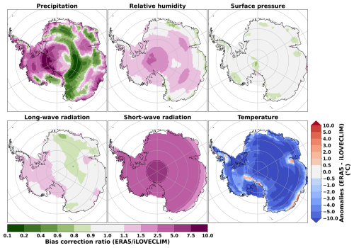
In fact, due to its coarse resolution and simplification in physics, iLOVECLIM displays some incorrect climate patterns. In particular, Heinemann et al. (2014) reported surface air temperature biases of iLOVECLIM compared to observations in North America and northern Europe, which are preserved in the downscaling version NH40 (Quiquet et al., 2018). To evaluate the impacts of these biases on the SMB simulation, we carry out a simple bias correction process by using ERA5 (Muñoz-Sabater et al., 2021), a set of reanalysis climate data, as reference (see Appendix C). In general, the variables with strong biases are total precipitation, shortwave radiation, and air temperature (Figs. C1 and C2). In addition, for the Antarctic Ice Sheet, the humidity is strongly underestimated in iLOVECLIM. These biases might partly come from simplified physics and the lack of explicit vertical representation in iLOVECLIM. For example, the clouds are prescribed based on the present-day climatology. These biases need further investigation in future works.

2.1.3 ITM standalone

In terms of the SMB scheme, iLOVECLIM uses the insolation temperature melt (ITM) method (Van Den Berg et al., 2008). This parameterization is implemented to provide the SMB to the ice sheet model embedded in iLOVECLIM, named GRISLI, for coupling purposes (Quiquet et al., 2021).

This parameterization calculates the runoff water (in mWE d⁻¹) as

$$\begin{array}{}\text{(1)}& \begin{array}{rl}{\displaystyle \frac{\partial m_{\text{runoff}}}{\partial t}}& ={\displaystyle \frac{\mathrm{1}}{{\mathit{\rho }}_{\mathrm{w}}{L}_{\mathrm{m}}}}\left(\right(\mathrm{1}-{\mathit{\alpha }}_{\mathrm{s}})\text{SW}\\ & +\text{crad}+\mathit{\lambda }(T_{\mathrm{air}}-\mathrm{273.15}))\ge \mathrm{0},\end{array}\end{array}$$

in which ρ_w is the liquid water density (1000 kg m⁻³), L_m is the specific latent heat of melting (3.34 × 10⁵ J kg⁻¹), α_s is the surface albedo, SW is the surface shortwave radiation (W m⁻²), and T_air is the near-surface air temperature (K). Meanwhile, λ and crad are two empirical parameters.

For the coupling between iLOVECLIM and GRISLI, Quiquet et al. (2021) implemented an albedo interpolation to take into account the altitude of the grid points (vertical) and to create a smooth transition of albedo value from ocean to land area (horizontal). In addition, to take into account the temperature bias of iLOVECLIM, a local modification of the parameter crad based on the annual mean temperature difference compared to ERA-Interim (Dee et al., 2011) is also included in ITM, as explained in Quiquet and Roche (2024).

Here, to provide a clean comparison to BESSI, a standalone version of ITM is used with the same albedo value as the ice grid points in iLOVECLIM (α_s = 0.85) and λ = 10 W m⁻² K⁻¹ as in Quiquet et al. (2021). The input data SW and T_s are read from BESSI input; hence, ITM also runs at a daily time step. The empirical parameter crad is tuned for the present-day climate with MAR as forcing. The SMB is the remaining total precipitation (accumulation) after subtracting the calculated runoff only (ablation), with the sublimation process being neglected.

2.2 Present-day climate reference data

For calibration/validation purposes, we use the present-day climate data from one of the state-of-the-art regional climate models: Modèle Atmosphérique Régional (MAR). MAR has been widely applied to study the SMB changes and surface melt for polar regions (Fettweis et al., 2017; Agosta et al., 2019; Mankoff et al., 2021). The model, with a typical sub-daily time step of 120 s (Fettweis, 2007), includes a 3D atmospheric model coupled with a 1D surface–atmosphere energy mass exchange scheme, the Soil–Ice–Snow–Vegetation–Atmosphere Transfer (SISVAT) (Fettweis et al., 2017), which is more complex and physical than BESSI. It can simulate up to 30 layers of snow/ice and consider snow properties and metamorphism (Kittel et al., 2021). Also, the simulated surface albedo takes into account more variables, including snow's optical properties, clouds, snow depth, the presence of bare ice, and liquid water (Tedesco et al., 2016). Detailed information about MAR and its setup can be found in Fettweis (2007) and Fettweis et al. (2013).

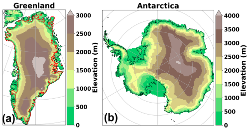
Figure 3 Topography of MAR for (a) Greenland (15 km × 15 km), with the present-day ice sheet extent in red contour, and (b) Antarctica (35 km × 35 km).

In this study, MAR acts as present-day forcing and reference benchmarks to compare with BESSI and ITM for both the Greenland and Antarctic ice sheets (denoted as GrIS and AIS, respectively). The resolution of the climate forcings is 15 km × 15 km for the GrIS (version 3.13) (Fig. 3a) and 35 km × 35 km for the AIS (version 3.12) (Fig. 3b), covering the period 1979–2021.

2.3 Study design

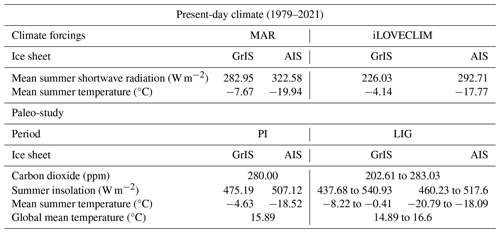
In this work, we carry out three sets of experiments corresponding to the two climate forcings: MAR for present-day conditions and iLOVECLIM for both present-day and LIG conditions. The climate characteristics of these experiments are presented in Table 1.

Table 1 Climate characteristics of two different climate forcings, MAR and iLOVECLIM, for different experiments. The calibration/validation is carried out from 1979 to 2021 with forcings from MAR and iLOVECLIM. The mean summer shortwave radiation and mean summer temperature are calculated based on the present-day ice sheet extent. The climate forcings for the Last Interglacial (LIG) comes from iLOVECLIM only. The summer insolation of the paleo-study corresponds to the summer insolation of 65° N for the Greenland Ice Sheet (GrIS) and 65° S for the Antarctic Ice Sheet (AIS). The summer months are June–July–August for the GrIS and December–January–February for the AIS.

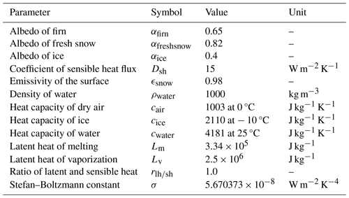
In the first experiment, we investigate the behaviors of BESSI and ITM for present-day climate by using MAR as forcing (BESSI-MAR and ITM-MAR). The calibration and validation are carried out for the GrIS and the AIS during the study period from 1979 to 2021, with the calibration carried out for the GrIS only. To evaluate the results, we use two goodness-of-fit metrics, which are the coefficient of determination R² and the root-mean-square error (RMSE), to assess the differences of BESSI-MAR and ITM-MAR with reference to MAR (see Appendix B). Initially, BESSI is spun up by looping the forcing several times until it reaches an equilibrium state. The ice mask corresponds to present-day ice sheet extent, classified in MAR as grid cells with more than 50 % of permanent ice. Some of BESSI's parameters related to albedo simulation (α_freshsnow, α_firn, and α_ice) and turbulent latent heat flux calculation ($r_{\mathrm{lh}/\mathrm{sh}}$ and D_sh) are tuned to obtain the lowest RMSE value between BESSI and MAR output and the narrowest gap in terms of the total SMB (SMB integrated over the ice sheet mask). The final values of these parameters are presented in Table A1. The same tuning procedure is applied for the empirical parameter crad of ITM, and the optimized value is −10 W m⁻².

Before applying BESSI and ITM for the LIG with iLOVECLIM as forcing, we investigate the influences of the input on the behavior of the two SMB models by comparing the results of BESSI-iLOVECLIM and ITM-iLOVECLIM to MAR for present-day conditions. iLOVECLIM forcings for the present day are obtained by running the model with the prescribed greenhouse gas (GHG) concentrations during the same period as MAR, from 1979 to 2021. As mentioned above (Sect. 2.1.2), we implement a simple bias correction process to correct the climate field of iLOVECLIM. To quantify the impact of these biases on the SMB simulation, in addition to original climate forcings, we also run BESSI and ITM with the bias-corrected version of iLOVECLIM.

For the LIG, to obtain the climate forcing, we run iLOVECLIM transiently from 135 to 115 ka, with present-day ice sheet topography and varying orbital configuration and concentrations of GHG. For every 500 years, we sample 50 years of daily output to provide forcings for BESSI and ITM. In total, there are 41 sets of inputs corresponding to 41 time slices covering the entire LIG. BESSI is spun up with the input data from the first time slice: 135 ka to reach the equilibrium state. Then, for each time slice, we run BESSI for 100 years with the snowpack from the spin-up and take the annual mean of the last 50 years for further analysis. The evolution of the SMB simulated by BESSI and ITM during the LIG is then compared to investigate the models' behaviors. In order to assess the trend of SMB evolution, we compute the differences in the annual mean SMB during the LIG with respect to the pre-industrial (PI) value for both BESSI-iLOVECLIM and ITM-iLOVECLIM. The climate forcing of the PI is obtained by running downscaled iLOVECLIM for 50 years from a 1000-year spin-up under pre-industrial boundary conditions. To quantify the biases of climate forcing on the models' behavior, assuming the biases in iLOVECLIM are constant with time, we use the present-day bias correction factors to correct the climate forcings for the LIG and the PI. The results of before and after the bias correction are then compared.

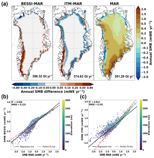
Figure 4 (a) Annual mean SMB anomalies (in mWE yr⁻¹) of BESSI-MAR and ITM-MAR compared to MAR for the Greenland Ice Sheet. The reference, MAR, is shown in absolute annual SMB values. The total SMB (in Gt yr⁻¹) integrated for the ice sheet area is also included. The scatter plots of (b) BESSI-MAR vs. MAR and (c) ITM-MAR vs. MAR indicate the SMB of each grid point (in mWE yr⁻¹) with elevation classification, including the linear regression line in black and the perfect-fit line (1,1) in red.

Figure 5 Contribution of different key processes to the 43-year mean total SMB of MAR, BESSI-MAR, and ITM-MAR in (a) Greenland and (b) Antarctica (in Gt yr⁻¹).

3 Results

3.1 MAR as present-day climate forcings

3.1.1 Greenland

The map of the annual mean SMB differences simulated by BESSI-MAR and ITM-MAR compared to MAR (shown in absolute value) for the Greenland Ice Sheet during the period 1979–2021 is presented in Fig. 4a. For BESSI-MAR, in the southwest of Greenland, there is a wide spread of positive SMB anomalies, indicating an underestimation of this ablation zone, which is also reported by Plach et al. (2018) and Fettweis et al. (2020) (Fig. S1 in the Supplement). Such high SMB values in BESSI-MAR for this area is related to the albedo simulation. Compared to MAR, the annual albedo simulated for the southwest of the GrIS is higher in BESSI-MAR, leading to a lower runoff rate (Fig. S2). Even though the extent is underestimated, the magnitude of ablation in BESSI-MAR is higher than MAR around the margins, particularly in the north and west of Greenland. For these grid points, BESSI-MAR simulates high melt rates, while the amount of water refreeze remains low (Fig. S3a, b), resulting in negative SMB anomalies compared to MAR. In the center of the ice sheet, where sublimation/evaporation is dominant due to dry climate, the SMB is simulated correctly by BESSI-MAR with reference to MAR. However, this process is slightly underestimated in some areas, notably the west of the ice sheet (Fig. S3c). In general, the 43-year mean SMB simulated by BESSI-MAR is in good agreement with MAR despite a simpler model structure, with a 2 % difference in the total SMB.

For ITM-MAR, the differences in the SMB compared to MAR come from the runoff simulation, as the model does not simulate other processes. Hence, the differences are located mostly in low-elevation areas, where the temperature is not low enough to compensate for the shortwave radiation influence (Eq. 1) during the summer months (Fig. S4a, b). Around the ice sheet margin, ITM-MAR simulates less runoff around the margins due to a constant albedo value (0.85) (Fig. S2), resulting in SMB overestimation for these grid points. The total SMB difference between ITM-MAR and MAR is around 6.64 %, 3 times more than that of BESSI-MAR.

The scatter plots of the grid points with different elevations in the SMB maps are also presented in Fig. 4, with evaluation metrics to illustrate the goodness of fit of BESSI-MAR and ITM-MAR to MAR. Compared to MAR, BESSI-MAR tends to underestimate the SMB of the low-elevation grid points located in the ice sheet margin in the north and west (Fig. 4b). For points located near the equilibrium line (with SMB ≈ 0), the SMB is slightly overestimated in BESSI-MAR. Meanwhile, ITM-MAR shows a trend of SMB overestimation for grid points located in the ablation area (Fig. 4c). In general, the evaluation metrics illustrate an acceptable SMB simulation of both BESSI-MAR and ITM-MAR with respect to MAR.

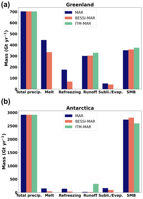
Figure 5a illustrates the mean value of total SMB elements simulated by the three models for the GrIS. For BESSI-MAR, we can see strong underestimations in melt and refreezing compared to MAR, especially refreezing with less than half of MAR's value. This might result from the daily time step, which causes the model to neglect the diurnal temperature cycle (Krebs-Kanzow et al., 2018). However, these underestimations are compensated in the runoff, leading to an acceptable value in BESSI-MAR compared to MAR. Meanwhile, the sublimation/evaporation rate in BESSI-MAR is slightly lower than MAR due to the underestimation of this process. For ITM-MAR, the model compensates for the absence of the sublimation/evaporation process by simulating more runoff to obtain a similar SMB rate compared to MAR. Both BESSI-MAR and ITM-MAR overestimate the SMB with reference to MAR. This trend is consistent during the study period (Fig. S5a).

3.1.2 Antarctica

The annual mean SMB differences in BESSI-MAR and ITM-MAR with respect to MAR for the Antarctic Ice Sheet are shown in Fig. 6a. For Antarctica, BESSI-MAR shows a high agreement with MAR on the SMB simulation with very limited differences. The problem related to melting in Greenland is limited here as it has a much colder climate (Fig. S6a), and sublimation/evaporation becomes dominant. The differences between the two models come from the underestimation of sublimation/evaporation around the ice sheet margin in BESSI-MAR (Fig. S6b), leading to the larger gap between BESSI-MAR and MAR for this process compared to the GrIS (Fig. 5)

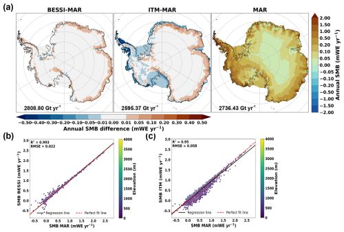
Figure 6 (a) Annual mean SMB anomalies (in mWE yr⁻¹) of BESSI-MAR and ITM-MAR compared to MAR for the Antarctic Ice Sheet. The reference, MAR, is shown in absolute annual SMB values. The total SMB (in Gt yr⁻¹) integrated for the ice sheet area is also included. The scatter plots of (b) BESSI-MAR vs. MAR and (c) ITM-MAR vs. MAR indicate the SMB of each grid point (in mWE yr⁻¹) with elevation classification, including the linear regression line in black and the perfect-fit line (1,1) in red.

Meanwhile, ITM-MAR exhibits large differences from MAR for the annual mean SMB. The anomalies located in the interior of the ice sheet come from the absence of sublimation/evaporation in this parameterization. The underestimation of the SMB around the edge of the ice sheet and the ice shelves comes from the high simulated runoff by ITM-MAR (Fig. S6a). ITM-MAR simulates runoff for these grid points due to high shortwave radiation that overweighs the mild temperature during the melting season (Fig. S7a, b). In terms of the total SMB, the differences between the two SMB models compared to MAR are in an acceptable range: 2.64 % for BESSI-MAR and −5.15 % for ITM-MAR (Fig.5b).

Similarly to the GrIS, scatter plots of the grid points with different elevations in the maps of Fig. 6a are also presented in Fig. 6b and c. For the AIS, there is no significant trend of under-/overestimation of the annual mean SMB in BESSI-MAR compared to MAR (Fig. 6b). On the other hand, ITM-MAR shows a strong SMB underestimation trend for low-elevation grid points (Fig. 6c) due to high runoff rates. These points correspond to the ablation zone over ice shelves that is not present in MAR. This trend is observed throughout the study period (Fig. S5b). The evaluation metrics suggest a good fit of the two SMB models to MAR, with BESSI-MAR having a slightly better value.

3.2 iLOVECLIM as climate forcing: present day

3.2.1 Greenland

iLOVECLIM has a coarser resolution and a simpler model setup than MAR: a state-of-the-art regional climate model used to calibrate/validate BESSI and ITM. This difference in the simulated climate strongly influences the behaviors of the two SMB models. The annual mean SMB during the period 1979–2021 simulated by BESSI-iLOVECLIM and ITM-iLOVECLIM for the GrIS is presented in Fig. 7a. Switching the climate forcings, the resolution of iLOVECLIM influences BESSI-iLOVECLIM significantly with the SMB patterns following the input field grid (Fig. S4). In particular, compared to BESSI-MAR for the same study period (Fig. S1), there are larger ablation zones in the south. Also, the magnitude of negative SMB in BESSI-iLOVECLIM is very high. This results from a warm climate of iLOVECLIM (Fig. C1) that induces high melt rates, while BESSI does not simulate the refreezing process well due to a large time step (as mentioned in Sect. 3.1.1). Consequently, the contribution of runoff to the total SMB in BESSI-iLOVECLIM is very high compared to MAR, as illustrated in Fig. 8a, leading to a much lower SMB value even for a higher total precipitation rate (89.38 Gt yr⁻¹ vs. 351.29 Gt yr⁻¹, respectively). On the other hand, due to the drier atmosphere (Fig. S4d), the sublimation/evaporation in BESSI-iLOVECLIM is more than twice as much as MAR's value.

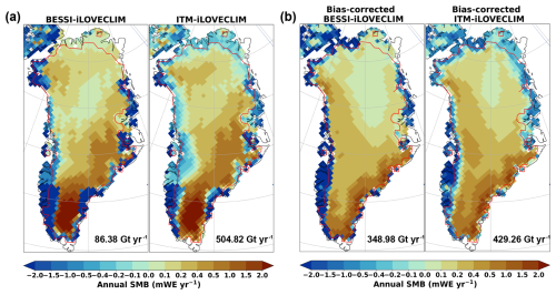
Figure 7 Comparison of the annual mean SMB (in mWE yr⁻¹) between BESSI-iLOVECLIM and ITM-iLOVECLIM (a) before and (b) after bias correction for Greenland Ice Sheet. The total SMB (in Gt yr⁻¹) integrated for the present-day ice sheet extent (red line) is also included.

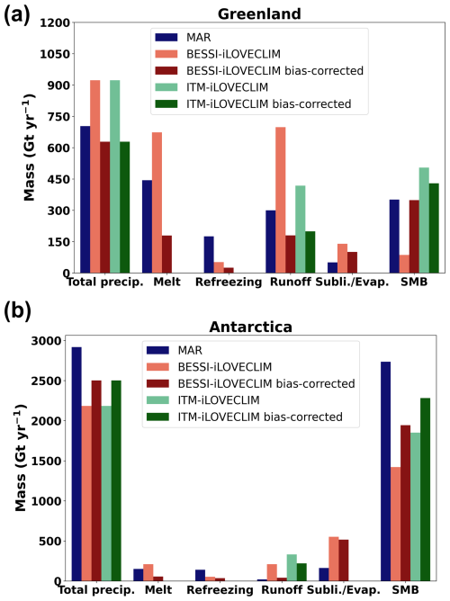
Figure 8 Comparison of the contribution of different key processes to the 43-year mean total SMB of BESSI-iLOVECLIM and ITM-iLOVECLIM before and after bias correction in (a) Greenland and (b) Antarctica with MAR as reference (in Gt yr⁻¹).

The climate forcing also strongly influences ITM-iLOVECLIM, with similarly large ablation zones in the south of the GrIS to those in BESSI-iLOVECLIM. However, the ablation zones in ITM-iLOVECLIM are larger than in BESSI, particularly in the southwestern and northern regions of Greenland. Therefore, the runoff contribution to the total SMB for ITM-iLOVECLIM is higher than for MAR (Fig. 8a). Despite a higher runoff value, ITM-iLOVECLIM still has a higher SMB value than that of MAR due to a higher total precipitation rate, as indicated in Figs. 7a and 8a.

As the biases in iLOVECLIM exhibit a strong influence on BESSI and ITM, the annual mean SMB simulated with a corrected climate forcing is presented in Fig. 7b. With the adjusted input, BESSI-iLOVECLIM simulates more appropriate SMB patterns with the narrow ablation zone in the southwest presence and a bigger extent of the low-accumulation zone in the center north of the ice sheet. For ITM-iLOVECLIM, similar patterns are observed with better illustration of the ablation zones as in ITM-MAR (Fig. S1). The contribution of different processes to the total SMB of bias-corrected BESSI-iLOVECLIM and ITM-iLOVECLIM is shown in Fig. 8a together with results from MAR and the original iLOVECLIM. Noticeably, the total precipitation after the bias correction in iLOVECLIM decreases from 923 to 629 Gt yr⁻¹, around 10.5 % lower than MAR's value (703 Gt yr⁻¹). This is the result of limiting the correction factors to be in the range of 0.1 to 10.0, which neglects extreme values. For BESSI-iLOVECLIM, as the climate is cooler after the bias correction, the runoff rate reduces to 180 Gt yr⁻¹, nearly 4 times less than before the bias correction (698 Gt yr⁻¹). Because of the higher humidity, the sublimation/evaporation rate decreases from 140 to 101 Gt yr⁻¹, nearly double the value of MAR (51 Gt yr⁻¹). For ITM-iLOVECLIM, the simulated runoff decreases from 418 to 200 Gt yr⁻¹ after the bias correction, which is due to the colder climate. Since there is a reduction in the total precipitation, the total SMB in ITM-iLOVECLIM also declines to 429.26 from 504.82 Gt yr⁻¹ (around 15 %), as shown in Fig. 7b. The results indicate the importance of the climate forcing quality on the results of the two SMB models.

3.2.2 Antarctica

For the AIS, the annual mean SMB from 1979–2021 simulated by BESSI-iLOVECLIM and ITM-iLOVECLIM is presented in Fig. 9a. Similarly to the GrIS, the patterns of climate fields, mostly total precipitation (Fig. S7), strongly influence the simulated SMB by the two SMB models. Noticeably, there are large ablation zones observed in the center west and some parts of the east of the ice sheet in BESSI-iLOVECLIM, caused by the very low humidity (Figs. C2 and S7d). As shown in Fig. 8b, this bias leads to unrealistic sublimation/evaporation simulation by BESSI-iLOVECLIM, around 3 times higher than in MAR (around 551 Gt yr⁻¹ compared to 162 Gt yr⁻¹). Figure 8b also indicates a low total precipitation rate of only 2184 Gt yr⁻¹ in iLOVECLIM, nearly 25 % lower than in MAR (2919 Gt yr⁻¹). The total SMB simulated by BESSI-iLOVECLIM for this ice sheet is around 1421.87 Gt yr⁻¹, around 50 % lower than in MAR (2736.43 Gt yr⁻¹). Meanwhile, the total SMB simulated by ITM-iLOVECLIM is 1851.77 Gt yr⁻¹. This rate is higher than in BESSI-iLOVECLIM and around 30 % lower than MAR's value. The contribution of runoff to the total SMB in ITM-iLOVECLIM for this ice sheet is relatively high, which is 332 Gt yr⁻¹ compared to 211 Gt yr⁻¹ for BESSI-iLOVECLIM.

Figure 9 Comparison of the annual mean SMB (in mWE yr⁻¹) between BESSI-iLOVECLIM and ITM-iLOVECLIM (a) before and (b) after bias correction for Antarctic Ice Sheet. The total SMB (in Gt yr⁻¹) integrated for the present-day ice sheet extent is also included.

The annual mean SMB simulated by BESSI and ITM with bias-corrected iLOVECLIM for the AIS is shown in Fig. 9b. For both the two models, the SMB patterns improve significantly with the corrected climate forcings. In BESSi-iLOVECLIM, the widespread ablation zones are removed. However, the bar chart indicates that the sublimation/evaporation in BESSI-iLOVECLIM remains three times higher than MAR's after the bias correction (Fig. 8b). For ITM-iLOVECLIM, runoff decreases slightly to 220 Gt yr⁻¹ (Fig. 8b). Such a high runoff contribution has also been observed before in ITM-MAR (Fig. 5). Despite the bias correction, the total precipitation in iLOVECLIM remains below the value of MAR due to the restriction range of the bias correction factor (see Appendix C). The gap is about 417 Gt yr⁻¹, which is around 14 % of the total precipitation in MAR. This leads to lower total SMB rates in both BESSI-iLOVECLIM and ITM-iLOVECLIM in comparison with MAR, with the difference being nearly −29 % in BESSI and around −17 % in ITM.

3.3 iLOVECLIM as climate forcing: Last Interglacial

3.3.1 Climate of the Last Interglacial

The external forcings of iLOVECLIM, including the summer insolation of 65° N and 65° S together with the carbon dioxide concentration, are presented in Fig. 10a. The range of these forcings for the LIG and the PI is also shown in Table 1. Figure 10b illustrates the evolution of simulated global mean temperature by iLOVECLIM during the LIG compared to the PI. The global mean temperature reaches a maximum value of 16.6 °C at around 128 ka, similar to the peak of carbon dioxide and 1000 years before the summer insolation of 65° N. The temperature difference between 127 ka and the PI in this work is 0.49 °C, which is at the upper end of the range −0.48 to 0.56 °C suggested by CMIP6/PMIP4 (Otto-Bliesner et al., 2021). The comparison of the simulated local temperature of iLOVECLIM and the temperature change proxy which reaches back to 123 ka at the North Greenland Ice Core Project (NGRIP) is shown in Fig. 10c. The simulated local surface temperature at NGRIP peaks at nearly the same time as the global mean temperature (around 128 ka). Meanwhile, the proxy-based data show a similar value around 6500 years later. This could result from the absence of ice sheet and climate interaction in our simulations, as the ice sheet component is not activated. The melting of the ice sheet could possibly delay the increase in temperature. The temperature difference between the LIG and the PI at NGRIP in our simulations is 4.2 °C, consistent with the range 5.2 ± 2.3 °C suggested by Landais et al. (2016). For Antarctica, the comparison of the simulated local surface temperature of iLOVECLIM and the temperature change proxy at EPICA Dome C (EDC) is presented in Fig. 10d. The change in the simulated temperature shows a good agreement with the proxy-based data regarding timing. However, the warming at EDC during the LIG compared to the PI in our work is only 0.59 °C, while the value suggested by Jouzel et al. (2007) is about 4.5 °C. This difference might result from the fixed ice sheet mask and topography in our simulations. It is possible that the West Antarctic Ice Sheet was smaller during the LIG, leading to a change in surface elevation and ice extent. This can, in turn, increase the temperature at EDC. This part of warming is not taken into account in our simulations.

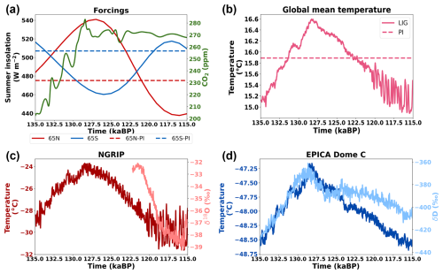
Figure 10 (a) Temporal variation in external forcings during the LIG: summer insolation of 65° N and 65° S (in W m⁻²) (Berger, 1978) and the carbon dioxide concentration (in ppm) (Lüthi et al., 2008). The dashed lines indicate summer insolation of the pre-industrial (PI). (b) Temporal variation in the 100-year mean of the global mean temperature (in degree Celsius) during the LIG with the value of the PI denoted by the dashed line. (c) The 100-year mean of the simulated local surface temperature (in degree Celsius) and δ¹⁸O (in ‰) (Andersen et al., 2004; Lemieux-Dudon et al., 2010) at the North Greenland Ice Project (NGRIP). (d) The 100-year mean of the simulated local surface temperature (in degree Celsius) and δD (in ‰) (Jouzel et al., 2007; Lemieux-Dudon et al., 2010) at EPICA Dome C (EDC). The proxy data include the impact of elevation changes, while our simulations do not.

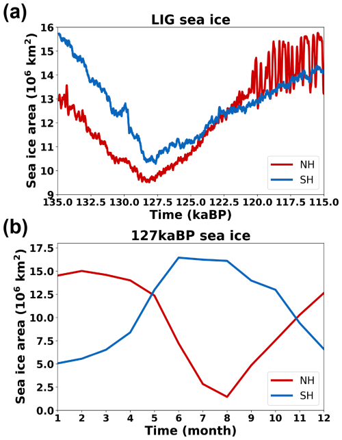
Figure 11 Simulated sea ice extent (in 10⁶ km²) for the Northern Hemisphere (NH) and Southern Hemisphere (SH) (a) during the LIG and (b) during 127 ka.

The simulated sea ice extent of the Northern Hemisphere and Southern Hemisphere (NH and SH, respectively) during the LIG is shown in Fig. 11a. For both hemispheres, the sea ice extent decreases during the LIG following the temperature changes, also reaching the minimum value around 128–127.5 ka. The evolution of sea ice extent of the two hemispheres during 127 ka in our simulation falls within the range suggested by CMIP6/PMIP4 (Fig. 4 in Otto-Bliesner et al., 2021).

3.3.2 Surface mass balance evolution during the Last Interglacial

Greenland

To study the evolution of the SMB during the LIG, we present the temporal variation in the annual mean total SMB and its sub-processes simulated by BESSI-iLOVECLIM for the GrIS in Fig. 12a. The rise in summer insolation in the north and the carbon dioxide concentration during the beginning of the LIG (Fig. 10a) induce an increase in the melt rate of Greenland (Fig. 12a). During the same period, the values of runoff are slightly higher than those of the melt, indicating that both rain and melt are not well refrozen due to the warm climate (Eq. A12). As the insolation drops after 127 ka, runoff and melt also decrease. In the same figure, total precipitation is shown to increase slightly during the insolation peak, which is expected as the climate gets warmer. Meanwhile, sublimation/evaporation remains stable throughout the period with a low magnitude, as this process is not dominant for the GrIS. Similarly, refreezing also remains low for this ice sheet; however, a slight increase during the peak of the LIG is observed in Fig. 12a. The total SMB in this case is mainly driven by runoff (melt), strongly decreases during the rise in summer insolation, and then recovers after 127 ka. At 128.5 ka, the total SMB shrinks to its minimum value (−1166 Gt yr⁻¹), which is much less than the SMB at the beginning of the LIG (74.33 Gt yr⁻¹).

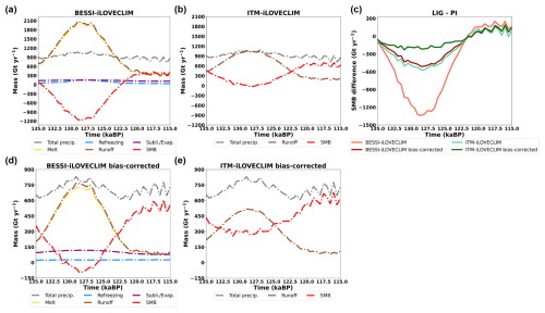
Figure 12 Temporal variation in the annual mean total SMB and its elements integrated on the present-day ice sheet extent during the LIG of (a) BESSI-iLOVECLIM and (b) ITM-iLOVECLIM (in Gt yr⁻¹) for Greenland. (c) Annual mean total SMB anomalies between the LIG and the pre-industrial of different cases. Panels (d) and (e) are similar to panels (a) and (b) but with bias-corrected iLOVECLIM.

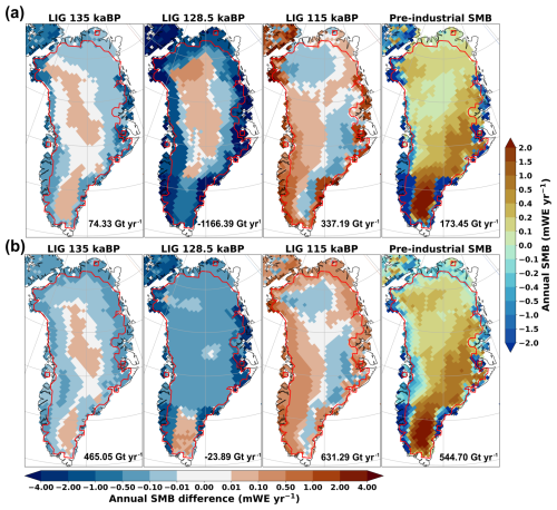
Figure 13 Annual mean SMB anomalies (in mWE yr⁻¹) between several LIG time slices (135, 128.5, and 115 ka) and the pre-industrial simulation of (a) BESSI-iLOVECLIM and (b) ITM-iLOVECLIM for the Greenland Ice Sheet. The absolute annual SMB value of the PI and the total SMB (in Gt yr⁻¹) integrated for the present-day ice sheet extent (red line) of each simulation is also included.

Similarly, the annual mean total runoff also increases following the increase in the external forcings in ITM-iLOVECLIM (Fig. 12b). However, the magnitude of the runoff is low, leading to the mostly positive total SMB values throughout the LIG. In particular, during the peak runoff (128.5 ka), the maximum runoff value simulated by ITM-iLOVECLIM is 1041.07 Gt yr⁻¹, about a half of BESSI's value during the same period (2030.66 Gt yr⁻¹).

By plotting the total SMB differences between the Last Interglacial and the pre-industrial periods simulated by the same model, we investigate the magnitude of SMB variation for both BESSI-iLOVECLIM and ITM-iLOVECLIM (Fig. 12c). During the peak of the LIG, the gap between the two models widens, with BESSI-iLOVECLIM much lower than ITM-iLOVECLIM. The difference between the two models reaches a value of nearly 770 Gt yr⁻¹ at 128.5 ka, when runoff reaches its peak for both models. As discussed above, the difference between the two models comes from the runoff simulation, which is also observed in the present-day climate conditions (Sect. 3.2.1)

To further investigate the differences between the two SMB schemes, the map of SMB anomalies of BESSI and ITM is shown in Fig. 13. In this figure, we select three different time slices from the LIG simulation, the first (135 ka), the peak of the runoff (128.5 ka), and the last (115 ka), to compare with the pre-industrial results. The pre-industrial annual mean SMB of the two models is quite similar to the present-day value (Fig. 7a). The two models display similar patterns for the first and last time slices of the LIG. Notably, at the beginning of the LIG, for the two models, positive SMB differences can be seen in the inner part of the ice sheet as there is more precipitation. Meanwhile, SMB rates around the margin are lower than the pre-industrial value, since the melting process accelerates due to warmer climate conditions. This SMB trend is enhanced during the peak of deglaciation (128.5 ka). In BESSI-iLOVECLIM, the magnitude of the negative differences around the margin is very high compared to ITM-iLOVECLIM, similar to the present-day climate condition (Fig. 7a). Additionally, BESSI-iLOVECLIM has larger ablation zones with very low SMB than ITM-iLOVECLIM, leading to a much lower total SMB rate in BESSI than in ITM (Fig. S8). In ITM-iLOVECLIM, grid cells with negative SMB anomalies compared to the PI are present in most parts of the ice sheet during 128.5 ka. The ablation zones simulated by this parameterization expand further into the center of the ice sheet (Fig. S8). Then, at the end of the LIG, both models simulate higher SMB rates around the margins, as a colder climate accelerates accumulation.

As the climate forcing strongly impacts the simulated SMB, similar runs of BESSI and ITM are carried out with input from the bias-corrected iLOVECLIM (Fig. 12d, e). With this bias-corrected forcing, the SMB simulated by BESSI-iLOVECLIM is systematically higher, consistent with the results obtained for the PI. The total SMB value at 135 ka (357.27 Gt yr⁻¹) is relatively close to that of the PI (415.75 Gt yr⁻¹). After that, the total SMB declines, becoming negative from 131 ka and reaching its minimum of −95.48 Gt yr⁻¹ at 128.5 ka. Then, the total SMB increases, becoming positive again from 125.5 ka and remaining above 500 Gt yr⁻¹ from 119 to 115 ka. The SMB simulated by ITM-iLOVECLIM follows a similar trend but with a much smaller magnitude. The minimum total SMB value is 270.95 Gt yr⁻¹ at 128.5 ka, around 40 % lower than 135 ka (436.07 Gt yr⁻¹). After that, the SMB rises and remains above 500 Gt yr⁻¹ from 120.5 to 115 ka. As the mean total SMB increases, the SMB gap between the LIG and the PI of BESSI and ITM also decreases (Fig. 12c). At the minimum peak of the SMB (128.5 ka), LIG–PI anomalies in BESSI-iLOVECLIM increases from −1340 to −511 Gt yr⁻¹. Meanwhile, for ITM, the magnitude of LIG–PI anomalies at 128.5 ka is about −215 Gt yr⁻¹, nearly one-half less than before the bias correction (−569 Gt yr⁻¹). The results suggest that ITM is less sensitive to the biases in iLOVECLIM than BESSI, which is also true for present-day experiments (Fig. 8a). After the bias correction, the simulated SMB patterns are improved for both SMB models, with a better pattern of SMB changes in the GrIS (Fig. S9).

Antarctica

Figure 14a and b illustrate the temporal variation in the annual mean total SMB and its sub-processes simulated by BESSI-iLOVECLIM and ITM-iLOVECLIM for the AIS. Compared to Greenland, during the same period, the annual mean values of the total SMB and its elements fluctuate less in Antarctica for both SMB models. In particular, in BESSI-iLOVECLIM, the total SMB at the peak of runoff (128 ka) is 1481.65 Gt yr⁻¹, nearly 13 % higher than the value of 135 ka (1312.72 Gt yr⁻¹). This number is very low compared to the magnitude of SMB differences in the GrIS. Also, the magnitude of the simulated annual mean total SMB by BESSI-iLOVECLIM during the LIG is quite low for the AIS (less than 2000 Gt yr⁻¹), which is due to the biases in humidity, as discussed in Sect. 3.2.2. During the LIG, even though the insolation at the South Pole decreases (Fig. 10a), the AIS still experiences an increase in the melt in BESSI-iLOVECLIM (Fig. 12a, b), which is caused by a higher global mean temperature (Fig. 10b). The sublimation is more dominant in the AIS than in the GrIS because of a much drier climate. Even though the sublimation is impacted by iLOVECLIM biases, no temporal change in this flux is simulated by the model. This suggests that the influences of the bias in the humidity of iLOVECLIM are constant. Due to this and the low value of runoff, for this ice sheet, the variation in the total SMB simulated by BESSI-iLOVECLIM follows the pattern of the total precipitation. It slightly increases as the global mean temperature increases, since a warmer climate induces more precipitation.

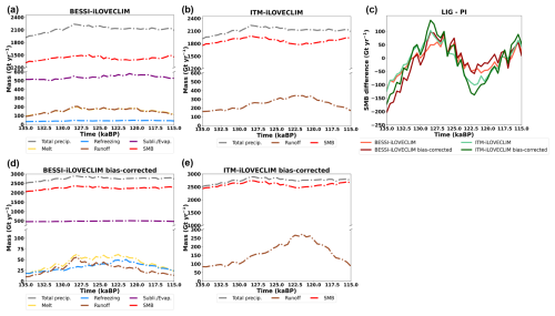
Figure 14 Temporal variation in the annual mean total SMB and its elements integrated on the present-day ice sheet extent during the LIG of (a) BESSI-iLOVECLIM and (b) ITM-iLOVECLIM (in Gt yr⁻¹) for Antarctica. (c) Annual mean total SMB anomalies between the LIG and the pre-industrial of different cases. Panels (d) and (e) are similar to panels (a) and (b) but with bias-corrected iLOVECLIM.

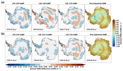
Figure 15 Annual mean SMB anomalies (in mWE yr⁻¹) between several LIG time slices and the pre-industrial simulation of (a) BESSI-iLOVECLIM and (b) ITM-iLOVECLIM for the Antarctic Ice Sheet. The absolute annual SMB value of the PI and the total SMB (in Gt yr⁻¹) integrated for the present-day ice sheet extent of each simulation are also included.

Similarly, the total SMB in ITM-iLOVECLIM for the AIS is also driven by the total precipitation. Even though the runoff rates in ITM are higher than in BESSI, the absence of sublimation/evaporation processes leads to high total SMB values in ITM-iLOVECLIM, which remain higher than 1700 Gt yr⁻¹ throughout the LIG. The simulated runoff increases following the increase in the global mean temperature and the summer insolation (Fig. 14b). Around 122.5–121.5 ka, the runoff rate reaches its peak of nearly 341 Gt yr⁻¹, about 2 times more than the value of 135 ka (159 Gt yr⁻¹).

Figure 14c indicates that the discrepancies between BESSI and ITM in terms of the SMB anomalies between the LIG and the PI are less significant for Antarctica than Greenland (Fig. 12c). As Fig. 14a indicates that sublimation/evaporation is almost constant during the LIG in BESSI-iLOVECLIM, the gap between the two models in Fig. 14c can only be explained by the differences in runoff simulation.

We also investigate the patterns of the annual mean SMB differences between several time slices of the LIG and the PI in the simulations of BESSI-iLOVECLIM and ITM-iLOVECLIM (Fig. 15). Similarly to the GrIS, the pre-industrial annual mean SMB of the two models is also consistent with the present-day results of the AIS (Fig. 9a). However, contrary to the GrIS, Fig. 15 suggests not much difference in the SMB value between the LIG and the PI and between the two models for this ice sheet. This is consistent with Fig. 14c, as the magnitude of the differences is very low compared to that of the absolute SMB value (Fig. S10).

For Antarctica, we also investigate the total SMB and its elements with the forcings from the bias-corrected iLOVECLIM (Fig. 14d, e). Noticeably, the simulated melt in BESSI-iLOVECLIM after bias correction reaches its peak at 128 ka and remains stable for 6000 years before gradually decreasing after 122.5 ka. The prolongation of high melt rates is related to the high global mean temperature (Fig. 10b) and the increase in summer insolation of 65° S during this period. The peak of refreezing at 122.5 ka indicates that the temperature gets colder, leading to the drop in the melt rate after this time slice (Fig. 14d). The magnitude of runoff decreases for both BESSI and ITM with the bias-corrected iLOVECLIM forcings due to the colder climate, leading to higher total SMB values (Fig. S11). Considering the magnitude of the total SMB in the AIS, Fig. 14c suggests the LIG–PI anomalies of the runs are not significant both before and after the bias correction.

4 Discussion

In this work, we assess the feasibility of replacing a parameterization scheme (ITM) with a physics-based surface energy balance model (BESSI) to provide a more physical SMB approach for the iLOVECLIM model framework to simulate the change in an ice sheet in the past.

The snow model, BESSI, performs well in the calibration/validation with MAR under the present-day climate. Highlighting the model's ability to simulate different climates faithfully, the first-ever simulation for Antarctica (without retuning) is in good agreement with MAR, which is more complex and has been intensively used to study this ice sheet. However, the issue related to the strong underestimation of refreezing (Plach et al., 2018; Born et al., 2019) remains (Fig. 5a). Lowering the time step of the model from daily to hourly might solve this problem, as the current model's large time step (daily) neglects the diurnal cycle of temperature (Krebs-Kanzow et al., 2018). On the other hand, the ablation simulated by BESSI is underestimated in extent but mostly overestimated in magnitude. In particular, the narrow ablation zone in the southwestern part of the GrIS is underestimated in BESSI-MAR compared to MAR (Fig. S1), which is also reported in Fettweis et al. (2020). However, due to the compensation of melt and refreezing, the results of the snow model are in good range with respect to MAR. On the other hand, the parameterization, ITM, needs individual tuning for the GrIS and the AIS. Hence, ITM-MAR, with the parameter crad calibrated for the GrIS, generates an unrealistic runoff rate for the AIS due to the change in climate conditions (e.g., higher shortwave radiation) (Figs. 6a and S6a). With a lower crad value, the runoff rates could be reduced to obtain a more suitable total SMB value for Antarctica (Fig. S12a).

For the paleo-study, both BESSI-iLOVECLIM and ITM-iLOVECLIM simulate the SMB evolution during the LIG following the change in the orbital configuration and carbon dioxide concentration. With the bias-corrected climate forcings, the simulated SMB during 130–125 ka by BESSI-iLOVECLIM of the GrIS is slightly higher than the results of MAR and BESSI-MAR from the work of Plach et al. (2018) (Fig. 12). This indicates that BESSI can provide reliable results when forced by iLOVECLIM (with bias correction), a climate forcing with lower resolution than MAR. On the other hand, compared to Sommers et al. (2021), the SMB simulated by BESSI-iLOVECLIM after the bias correction is slightly higher during 127–123 ka for the GrIS. The reason for this is the missing interactive elevation and ice sheet mask. As in this work, we use the present-day ice sheet topography and extent for all the experiments, leading to the absence of melt elevation feedback. Meanwhile, the total SMB simulated by ITM for the GrIS remains mostly positive throughout the LIG for both original and bias-corrected iLOVECLIM forcings. This suggests that the parameterization is unable to give suitable results without retuning its empirical parameters. As the runoff in ITM is calculated solely by one equation (Eq. 1), it is easy to have a desired runoff range by tuning its empirical parameters such as crad (Fig. S12a). Also, the albedo in ITM is fixed at 0.85, which is the value of ice grid points in iLOVECLIM, to give a clean comparison to BESSI. This can also be the reason behind the low-runoff simulation in ITM-iLOVECLIM during the LIG. A lower albedo value, which means more solar radiation is considered, can increase the simulated runoff rate of ITM (Fig. S12b). However, using only one albedo value for the whole ice sheet is not realistic. ITM with a range of albedo for different altitudes and locations can provide satisfying results, as in Quiquet et al. (2021).

The results of Sect. 3.2 indicate that the quality of the forcings strongly influences both BESSI and ITM. However, the changes in the simulated SMB by ITM-iLOVECLIM before and after bias correction are not as significant as in BESSI-iLOVECLIM for both ice sheets. The same behaviors of the two models are observed in the results of Sect. 3.3.2. The LIG results suggest that BESSI has higher sensitivity to the climate conditions, both with original and bias-corrected iLOVECLIM forcings. This suggests that ITM needs to be retuned whenever there is a change in the climate forcing in order to obtain desired values. However, this can be problematic for studies focusing on the paleo-periods that are not well documented. Also, a critical limitation of ITM is the missing sublimation/evaporation processes, which resulted in runoff overestimation. For BESSI, the runoff calculation is more realistic, and more processes are included than just solar radiation and heat. Hence, tuning BESSI is more complicated, as it is more physically constrained. Replacing ITM with BESSI to provide SMB to the ice sheet model GRISLI in iLOVECLIM framework can produce more physical results. Nonetheless, BESSI requires more input variables than ITM, making it more sensitive to the biases in iLOVECLIM, such as humidity. BESSI is also more computationally expensive (30 years per minute for the T21 grid) than a parameterization like ITM. However, considering the computational cost of iLOVECLIM (500 years per day), the extra cost of having BESSI instead of ITM in the framework is relatively small. In addition, we can be more confident in its response to a change in climate, since it explicitly simulates many processes, unlike ITM.

As in any climate model, iLOVECLIM displays some biases which can be locally dominant (Heinemann et al., 2014). In this work, we investigate the impact of these biases by using a simple delta method to correct the climate of iLOVECLIM (see Appendix C). The results of experiments with iLOVECLIM as climate forcings indicate the substantial impacts of these biases on the SMB simulation of both BESSI and ITM. In particular, the high temperature provided by iLOVECLIM leads to excessive runoff rates for both ice sheets, as shown in Sect. 3.2. However, transient LIG climate forcings can be obtained with much more favorable computational efficiency thanks to a simple model setup of iLOVECLIM. The results of the SMB models are significantly improved with the bias-corrected climate forcings. This suggests that there can be further improvement with a more sophisticated bias correction method.

5 Conclusions

This work examines the feasibility of replacing the SMB scheme of the Earth system model of intermediate complexity iLOVECLIM from a simple parameterization (ITM) with a physics-based surface energy balance model (BESSI) for the purpose of improving the simulation of ice sheet–climate interaction. For this purpose, a comparison between BESSI and ITM standalone is carried out for different climate forcings and climate conditions. Both BESSI and ITM provide acceptable results in the validation of the present-day period by MAR, a state-of-the-art regional climate model that includes a full physical energy mass transfer scheme of the surface for two very different ice sheet climate conditions: the GrIS and the AIS. For a paleoclimate study, the Last Interglacial period, climate fields simulated by an EMIC called iLOVECLIM are used as forcings for both SMB models. iLOVECLIM displays a large-scale climate change consistent with the forcings that translate to SMB evolution in agreement with previous modeling work. Switching from MAR to iLOVECLIM highlights the strong influence of the climate forcings on the simulation of the SMB evolution. In particular, iLOVECLIM presents important bias that leads to some significant misrepresentation of present-day SMB for both the GrIS and the AIS. These unrealistic climate patterns hamper the performance of both BESSI and ITM, posing the need for bias correction of the climate fields in iLOVECLIM. Notably, the comparison between BESSI and ITM during the Last Interglacial suggests a stronger sensitivity of BESSI to the climate conditions. The current SMB scheme of iLOVECLIM needs to be retuned for different climate forcings and study periods, which is not ideal for application in paleo-studies. Also, the absence of sublimation/evaporation processes in ITM leads to the overestimation of runoff in order to provide SMB in an acceptable range. The results suggest BESSI can be used to replace ITM, as this snow model maintains the low computational cost of iLOVECLIM while providing more reliable results without the need to be retuned.

Appendix A: BESSI model

In the following, we only detail the methodology used for surface energy and mass balance. Full details on the implementation of heat diffusion and snow mass compaction are given in Born et al. (2019).

Surface energy balance

The exchange of energy between the surface (the top layer of the model) and the atmosphere results in the change in temperature in this layer (T_s), influenced by the net solar flux Q_SW, the net longwave radiation flux Q_LW, the sensible heat flux Q_SH, the latent heat flux Q_LH, the heat flux from the precipitation Q_precip, and the melting flux Q_melt (when temperature reaches the melting point). This can be expressed as follows:

$$\begin{array}{}\text{(A1)}& \begin{array}{rl}{c}_{\text{ice}}{m}_{\text{top}}{\displaystyle \frac{\partial T_{\mathrm{s}}}{\partial t}}{|}_{\text{surface}}=& Q_{\text{SW}}+Q_{\text{LW}}+Q_{\text{SH}}+Q_{\mathrm{LH}}\\ & +Q_{\text{precip}}+Q_{\text{melt}},\end{array}\end{array}$$

in which c_i is the heat capacity of ice (2110 J kg⁻¹K⁻¹ at −10 °C) and m_top is the mass of the top layer in kg m⁻².

The net incoming solar radiation Q_SW is calculated from the albedo of the surface (α_snow or α_ice) and the incoming shortwave radiation F_SW (Wm⁻²) available from the forcing:

$$\begin{array}{}\text{(A2)}& Q_{\text{SW}}=(\mathrm{1}-\mathit{\alpha })F_{\text{SW}}.\end{array}$$

The albedo of ice α_ice is fixed at 0.4, while the albedo of snow α_snow is calculated considering the exponential decay with time since the last snowfall event (Oerlemans and Knap, 1998; Zolles and Born, 2021):

$$\begin{array}{}\text{(A3)}& {\mathit{\alpha }}_{\text{snow}}={\mathit{\alpha }}_{\text{firn}}+({\mathit{\alpha }}_{\text{freshsnow}}-{\mathit{\alpha }}_{\text{firn}})\exp \left({\displaystyle \frac{-N_{\text{snowfall}}}{t^{*}}}\right),\end{array}$$

in which the albedo of firn α_firn is 0.6, the albedo of the fresh snow α_freshsnow is 0.82, N_snowfall is the number of days since the last snowfall event, and t^* is the number of days for the fresh snow to reach firn condition. Depending on the temperature of the surface T_s, t^* is set to 20 d for T_s<273.15 K or 5 d for T_s=273.15 K.

Table A1 Table of physical constants and model parameters of the BESSI model.

The difference between the upcoming longwave radiation F_LW from the atmosphere (read from the input) and the emitted longwave radiation flux is the net longwave radiation Q_LW:

$$\begin{array}{}\text{(A4)}& Q_{\text{LW}}=F_{\text{LW}}-\mathit{\sigma }{\mathit{ϵ}}_{\mathrm{s}}{T}_{\mathrm{s}}^{\mathrm{4}},\end{array}$$

in which σ is the Stefan–Boltzmann constant (5.670373 × 10⁻⁸ W m⁻² K⁻⁴) and ϵ_s is the emissivity of the snow (0.98).

The turbulent sensible heat flux Q_SH is equal to the difference between the temperature of the air T_air and that of the surface layer T_s multiplied by a coefficient D_sh (15 W m⁻² K⁻¹):

$$\begin{array}{}\text{(A5)}& Q_{\text{SH}}=D_{\mathrm{sh}}(T_{\mathrm{air}}-T_{\mathrm{s}}).\end{array}$$

The turbulent latent heat flux Q_LH depends on the difference between the water vapor pressure of the air e_air and of the surface layer e_s, the surface pressure p_air from input, and a coefficient D_lh:

$$\begin{array}{}\text{(A6)}& {\displaystyle }& {\displaystyle }{Q}_{\mathrm{LH}}={\displaystyle \frac{D_{\mathrm{lh}}}{p_{\mathrm{air}}}}(e_{\mathrm{air}}-e_{\mathrm{s}}),\text{(A7)}& {\displaystyle }& {\displaystyle }\text{ with }{D}_{\mathrm{lh}}=\mathrm{0.622}{r}_{\mathrm{lh}/\mathrm{sh}}{\displaystyle \frac{D_{\mathrm{sh}}}{c_{\mathrm{air}}}}(L_{\mathrm{v}}+L_{\mathrm{m}}),\end{array}$$

where $r_{\mathrm{lh}/\mathrm{sh}}$ is the ratio of the exchange rates between the latent heat and sensible heat (equal to 1.0 in this work) and c_air is the heat capacity of the air (1003 J kg⁻¹ K⁻¹ at 0 °C), whilst L_v and L_m are latent heat of vaporization and melting, respectively (2.5 × 10⁶ and 3.34 × 10⁵ J kg⁻¹). Details of the turbulent sensible and latent heat flux calculation methods are available in Zolles and Born (2021).

Based on the air temperature (T_air), BESSI classifies total precipitation as snow (T_air≤273.15 K) or rain (T_air>273.15 K). When snow/rain falls, the air temperature is transported to the surface. Hence, the equations of heat flux from the snow/rain are

$$\begin{array}{}\text{(A8)}& {\displaystyle }& {\displaystyle }{Q}_{\text{precip,s}}=m_{\text{precip}}{c}_i(T_{\mathrm{air}}-T_{\mathrm{s}}),\text{(A9)}& {\displaystyle }& {\displaystyle }{Q}_{\text{precip,r}}=m_{\text{precip}}{c}_w(T_{\mathrm{air}}-\mathrm{273.15}),\end{array}$$

where m_precip is the mass of precipitation (kg m⁻² d⁻¹) and c_water is the heat capacity of water (4181 J kg⁻¹ K⁻¹ at 25 °C).

The model uses an implicit scheme for which the energy fluxes are calculated first, followed by the energy required to heat the top layer to the melting point. As the temperature of the surface cannot exceed the melting point, the remaining energy is regarded as energy available to melt snow/ice Q_melt (Eq. A1). The main parameters of the model are presented in Table A1.

Surface mass balance

The surface mass balance (SMB) is an important element of the ice sheet mass balance, apart from the ice discharge and basal melting. In BESSI, the SMB is calculated as the remaining mass of total precipitation from runoff and sublimation/evaporation processes:

$$\begin{array}{}\text{(A10)}& {\displaystyle }\text{SMB}=m_{\text{precip}}-(m_{\text{runoff}}+m_{\text{sub}}).\end{array}$$

In BESSI, the incoming precipitation (rain/snow) accumulates first on the surface (Fig. 1). Generally, the precipitation adds snow mass to the top snow layer (T_air≤273.15 K) or liquid mass to the water content of the surface (T_air>273.15 K). As more snow accumulates in the top layer, BESSI generates new snow layers below to prevent the mass of the layer from exceeding the maximum threshold (500 kg m⁻²). The mass of the new layer is set at 300 kg m⁻², and the old layer keeps the remaining mass, continuing to accumulate snow. Depending on the precipitation and the temperature, up to 15 layers can be formed. When more than one layer exists, the masses of these layers are shifted down to leave space for the newly forming layer. In contrast, when Q_melt is available, the snow column melts from the top. To prevent the mass of the surface layer from sinking below the minimum threshold (100 kg m⁻²), BESSI merges this layer with the next one. After the merging, the masses of the layers below are shifted up. In cases where Q_melt is enough to melt all the snow layers, ice starts to melt, adding water to the runoff.

The water resulting from melt and rain is retained by the snow column up to 10 % of its pore volume. The excess water percolates through the snow column, either refreezing due to low temperatures or leaving the lowest layer as runoff. The energy for refreezing, according to the assumption that the snow and the liquid water inside the snowpack are in thermodynamic equilibrium (Born et al., 2019), is calculated as

$$\begin{array}{}\text{(A11)}& Q_{\text{refreezing}}=c_i{m}_{\mathrm{s}}(\mathrm{273.15}-T_{\text{snow}}),\end{array}$$

in which T_snow is the temperature of the snow layer where the process takes place. Refreezing can occur anywhere among the snow layers, unlike melt, which happens only at the top.

The resulting amount of water from processes of rain, melt, and refreezing that leaves the bottom layer is regarded as runoff:

$$\begin{array}{}\text{(A12)}& {\displaystyle \frac{\partial m_{\text{runoff}}}{\partial t}}=m_{\text{rain}}+m_{\text{melt}}-m_{\text{refreezing}}\ge \mathrm{0}.\end{array}$$

Sublimation/evaporation, depending on the humidity of the air, is converted from the turbulent latent heat flux Q_LH to mass as

$$\begin{array}{}\text{(A13)}& {\displaystyle \frac{\partial m_{\text{sub}}}{\partial t}}=-{\displaystyle \frac{Q_{\mathrm{LH}}}{L_{\mathrm{v}}+L_{\mathrm{m}}}}.\end{array}$$

Positive values indicate sublimation/evaporation happens, subtracting mass from the SMB. On the contrary, deposition/condensation occurs, adding mass to the SMB.

Appendix B: Evaluation metrics for BESSI-MAR and ITM-MAR with MAR as climate forcing

The goodness-of-fit metrics used to evaluate behaviors of BESSI-MAR and ITM-MAR for the present-day climate conditions are presented in the following. The coefficient of determination R² is calculated as

$$\begin{array}{}\text{(B1)}& {\displaystyle }{R}^{\mathrm{2}}=\mathrm{1}-{\displaystyle \frac{{\sum }_i^n(X_{{\text{BESSI}}_i}-X_{{\text{MAR}}_i}{)}^{\mathrm{2}}}{{\sum }_i^n(X_{{\text{MAR}}_i}-\stackrel{\mathrm{‾}}{X_{\text{MAR}}}{)}^{\mathrm{2}}}},\end{array}$$

in which $(X_{{\text{BESSI}}_i}-X_{{\text{MAR}}_i})$ is the difference between the climatological annual mean value of the same variable of BESSI-MAR and MAR for the grid cell i. $\stackrel{\mathrm{‾}}{X_{\text{MAR}}}$ indicates the spatial mean value of MAR in the 43-year mean result.

The root-mean-square error (RMSE) is defined as

$$\begin{array}{}\text{(B2)}& {\displaystyle }\text{RMSE}=\sqrt{{\displaystyle \frac{\mathrm{1}}{n}}\sum _i^n(X_{{\text{BESSI}}_i}-X_{{\text{MAR}}_i}{)}^{\mathrm{2}}}.\end{array}$$

Here, n is the total number of grid points of each ice sheet domain, 7665 for the GrIS and 11 217 for the AIS, which is also the case for Eq. (B1). The same equations are applied to ITM-MAR.

Appendix C: Bias correction procedure for iLOVECLIM

To investigate the influence of the climate biases in iLOVECLIM on BESSI and ITM behaviors, we use the delta method to correct these biases with ERA5 (Muñoz-Sabater et al., 2021), a set of reanalysis climate data, as reference.

Input for BESSI includes near-surface temperature, precipitation, surface pressures, humidity, and short-/longwave radiation in a daily time step. For temperature, the bias-corrected data are obtained as follows:

$$\begin{array}{}\text{(C1)}& {\displaystyle }{T}_{\mathrm{iLC}}{}^{\prime }=T_{\mathrm{iLC}}+(\stackrel{\mathrm{‾}}{T_{\text{ERA5}}}-\stackrel{\mathrm{‾}}{T_{\mathrm{iLC}}}),\end{array}$$

in which T_iLC^′ is the bias-corrected daily temperature of iLOVECLIM, T_iLC is the origin daily output of iLOVECLIM, and $(\stackrel{\mathrm{‾}}{T_{\text{ERA5}}}-\stackrel{\mathrm{‾}}{T_{\mathrm{iLC}}})$ is the difference in the daily climatological mean temperature of the period 1979–2021 between ERA5 and iLOVECLIM.

For other input variables, the bias correction is carried out as

$$\begin{array}{}\text{(C2)}& {\displaystyle }{X}_{\mathrm{iLC}}{}^{\prime }=X_{\mathrm{iLC}}\times {\displaystyle \frac{\stackrel{\mathrm{‾}}{X_{\text{ERA5}}}}{\stackrel{\mathrm{‾}}{X_{\mathrm{iLC}}}}},\end{array}$$

in which X_iLC^′ is the bias-corrected daily data of iLOVECLIM, X_iLC is the origin daily output of iLOVECLIM, and $\stackrel{\mathrm{‾}}{X_{\text{ERA5}}}$ and $\stackrel{\mathrm{‾}}{X_{\mathrm{iLC}}}$ are the daily climatological mean data of the period 1979–2021 corresponding to the reference (ERA5) and iLOVECLIM.

In order to avoid extreme value, the ratio ${\displaystyle \frac{\stackrel{\mathrm{‾}}{X_{\text{ERA5}}}}{\stackrel{\mathrm{‾}}{X_{\mathrm{iLC}}}}}$ is limited to be in the range of 0.1 to 10.0. In addition, for relative humidity only, once the bias is corrected, the value is restricted between 0.15 and 1.0 (15 %–100 %) to avoid unrealistic values. These bias correction factors are presented in Fig. C1 for the GrIS and Fig. C2 for the AIS.

Figure C1 Mean values of bias correction factors of iLOVECLIM with respect to ERA5 for Greenland.

Figure C2 Mean values of bias correction factors of iLOVECLIM with respect to ERA5 for Antarctica.