Insights into the Australian mid-Holocene climate using downscaled climate models

The mid-Holocene climate of Australia and the equatorial tropics of the Indonesian–Australian monsoon region is investigated using the Community Earth System Model (CESM) and the Weather Research and Forecasting (WRF) model. Each model is used to simulate the pre-industrial (1850) and the mid-Holocene (6000 years before 1950) climate. The results of these four simulations are compared to existing bioclimatic modelling of temperature and precipitation. The finer-resolution WRF simulations reduce the bias between the model and bioclimatic data results for three of the four variables available in the proxy data set. The model results show that temperatures over southern Australia at the mid-Holocene and in the pre-industrial period were similar, and temperatures were slightly warmer during the mid-Holocene over northern Australia and into the tropics compared to the pre-industrial. During the mid-Holocene, precipitation was generally reduced over northern Australia and in the Indonesian–Australian monsoon region, particularly during summertime. The results highlight the improved value of using finer-resolution models such as WRF to simulate the palaeoclimate.

1 Introduction

The Holocene is the current geological epoch that started following the Younger Dryas and cessation of glacial conditions 11.7 ka. The mid-Holocene corresponds to 6 ka and was a time when sea levels and greenhouse gas concentrations were roughly like present-day conditions. However, solar insolation was different due to changes in the Earth's orbital parameters (Berger and Loutre, 1991). The largest difference was the latitudinal and seasonal distribution of solar irradiance stemming from the larger obliquity and the timing of perihelion, which occurred at the austral spring equinox compared to near the austral summer equinox in present-day conditions (Otto-Bliesner et al., 2020).

These small but important differences in climatic conditions, combined with reasonable repositories of proxy palaeoclimate evidence, are why the mid-Holocene has been a baseline experiment as part of the Palaeoclimate Modeling Intercomparison Project (PMIP) and the subject of extensive analysis using global circulation models (GCMs) and Earth system models (ESMs) (Joussaume et al., 1999; Braconnot et al., 2007; Brierley et al., 2020). From the large collection of simulations of the mid-Holocene climate within the PMIP framework, there has been comprehensive analysis of the global conditions, which continues to improve as models become more sophisticated (Brierley et al., 2020). In association with this analysis, the mid-Holocene climate of Australia and the monsoon tropics to the north have also received attention as part of global analyses (Brierley et al., 2020), monsoon dynamics (D'Agostino et al., 2020; Jiang et al., 2015; Zhao and Harrison, 2012), and over drylands (Liu et al., 2019), using the ensemble of simulations produced through the PMIP framework. The consensus of this prior work was that the mid-Holocene over Australia was slightly cooler by up to 0.3 °C (Brierley et al., 2020). The cooling was more intense in the austral summer by up to 1 °C but mildly warmer in the austral winter, although not over the whole continent, with a mild cooling in the south (Brierley et al., 2020). Monsoon precipitation in the Australian tropics was likely reduced by up to 200 mm yr⁻¹ (D'Agostino et al., 2020) and shifted equatorward during the mid-Holocene (Jiang et al., 2015). Within the interior of Australia there was very little difference in the extent of dryland environments between the mid-Holocene and present day, although there was a slight expansion in “arid” conditions over the central and north-western regions of the continent (Liu et al., 2019).

The summation of the mid-Holocene Australian palaeoclimate from the modelling community contrast with bioclimatic analyses of the mid-Holocene summarised in the OZ-INTIMATE series (Reeves et al., 2013a). In this series, Reeves et al. (2013a) found that the early to mid-Holocene experienced the warmest temperatures before these temperatures declined in the late Holocene and that precipitation likely peaked by the mid-Holocene before decreasing and becoming more variable, which was linked to the intensification of El Niño in the late Holocene. Tropical precipitation is believed to have been slightly reduced during the mid-Holocene, which was linked to the northward propagation of the Intertropical Convergence Zone (Reeves et al., 2013a). Herbert and Harrison (2016) developed a pollen-based palaeoclimate data set for Australia, following the seminal work of Bartlein et al. (2011). This data set has since been expanded to include 239 sites across Australia (Annika Herbert, personal communication, 2020), which provides a basis for palaeoclimate model–data intercomparison.

Using quantified climate proxy data can help to inform an interpretation of the climate modelling results and provide a means of assessing the model skill in representing past climates. This kind of analysis, while extensive over Northern Hemisphere climates (e.g. Braconnot et al., 2012) where there are data (Bartlein et al., 2011), has not been tested over Australia. This presents an obvious opportunity to simulate the palaeoclimate of Australia and to analyse this in relation to the newly developed pollen proxy data set from Herbert and Harrison (2016).

In addition to the identified gap in the model–proxy data intercomparison research, there is a further possibility for the improvement of the simulated climate of Australia using downscaled models. Using regional climate models (RCMs) to simulate the present-day climate is widespread, although less so for simulating the palaeoclimate (Ludwig et al., 2019). Simulations of the mid-Holocene palaeoclimate have only been performed over Europe (Russo et al., 2022; Strandberg et al., 2022, 2014; Armstrong et al., 2019; Russo and Cubasch, 2016; Brayshaw et al., 2011), North America (Diffenbaugh and Sloan, 2004; Diffenbaugh et al., 2003), Asia (Paeth et al., 2019; Kim and Kim, 2014; Yu et al., 2014; Polanski et al., 2012; Liu et al., 2010; Zheng et al., 2007, 2004; Kim et al., 2005; Huo et al., 2021), Africa (Patricola and Cook, 2007), and New Zealand (Ackerley et al., 2013). The early work using downscaled climate models employed modifications to the insolation and greenhouse gas concentrations of the mid-Holocene climate and a resolution of ca. 50 km. As the field has evolved, research has begun to interrogate the influence of vegetation as a boundary condition (e.g. Ludwig et al., 2017; Strandberg et al., 2014, 2022) and use available bioclimatic proxy evidence to validate the modelling results (Ludwig et al., 2017; Russo et al., 2024; Strandberg et al., 2022). There is evidence that some improvement in the simulated climate can be achieved using finer-resolution models (Armstrong et al., 2019; Ludwig et al., 2017), particularly hydrological processes (Ludwig et al., 2019), and that vegetation plays an important role in the simulation of the palaeoclimate (Strandberg et al., 2022). These improvements stem from the better depiction of feedback and physical processes at the regional scale (Armstrong et al., 2019; Ludwig et al., 2017). Here we analyse the mid-Holocene palaeoclimate of Australia using both an ESM and RCM to evaluate the skill of both models with respect to bioclimatic modelled proxy data. Numerical modelling also allows the palaeoclimate of large regions of Australia to be simulated where palaeo-bioclimatic data are scarce or unavailable (Reeves et al., 2013a). These simulations provide the first downscaled palaeoclimate analysis of the mid-Holocene in Australia and insight into the climate that would have been experienced by early human populations.

2 Data and methods

To investigate the palaeoclimate of the mid-Holocene (MH), two simulations were performed: pre-industrial (1850 Common Era) control (PI) and 6 ka. These two simulations were performed with the Community Earth System Model (CESM) (Hurrell et al., 2013), which were then downscaled over an Australian domain using the Weather Research and Forecasting model (WRF) (Skamarock et al., 2021). The greenhouse gas concentrations and orbital parameters used in each simulation were modified and are shown in Table 1. The radiative forcing anomaly resulting from the slight differences between the MH and PI greenhouse gas concentrations was 0.54 W m⁻² (Etminan et al., 2016). The orbital parameters affect the seasonal and latitudinal distribution and the magnitude of insolation at the top of the atmosphere. At the MH period, the perihelion occurred near the austral spring equinox, compared to slightly after the austral summer solstice at the PI period. This change in the timing of the perihelion, combined with the small differences in the obliquity and eccentricity, resulted in strong positive insolation anomalies during the austral winter through to the austral spring over Australia, followed by negative anomalies during the austral summer and autumn (Fig. 1).

Table 1 The boundary conditions and orbital parameters for the pre-industrial and mid-Holocene simulations.

Figure 1 Seasonal cycle of insolation anomalies for the mid-Holocene minus pre-industrial periods (W m⁻²).

2.1 Earth system model

The Community Earth System Model (CESM) version 1.2 (Hurrell et al., 2013) was used to provide the coarse-resolution lateral boundary conditions for the regional climate modelling. CESM is a fully coupled Earth system model that used the Community Atmosphere Model v5.3 with 30 atmospheric layers and the Community Land Model v4.0 at a horizontal resolution of 1.9° latitude by 2.5° longitude. The ocean and ice components were the Parallel Ocean Program (POP) and Community Ice CodE (CICE) at a nominal 1° latitude and longitude. The PI and MH simulations were performed for 31 years, starting from climatically stable restart positions provided by the National Center for Atmospheric Research (NCAR), using only the last 30 years for analysis. To ensure that the model was in equilibrium, we checked the residual top-of-the-model radiation balance, which was 0.11 W m⁻² for PI and 0.12 W m⁻² for MH. CESM and its predecessor, the Community Climate System Model (CCSM), have been shown to provide suitable simulations of the palaeoclimate (Brady et al., 2013; Otto-Bliesner et al., 2020) and are representative of other models that have participated in the PMIP (Brierley et al., 2020; Harrison et al., 2015). CESM provided 6 h atmospheric boundary condition data, daily sea surface temperature and sea ice cover, and monthly average surface data required by the regional climate model.

2.2 Regional climate model

The downscaled regional climate model used was the WRF model version 4.4 (Skamarock et al., 2021). The WRF model is a dynamic climate model that solves the non-hydrostatic Euler equations with terrain-following vertical coordinates (Skamarock et al., 2021). WRF has been developed by NCAR and used extensively for research and commercial applications in numerical weather prediction (Skamarock et al., 2021). In palaeoclimate modelling, WRF has been used successfully in Europe (Russo et al., 2024; Velasquez et al., 2022, 2021; Stadelmaier et al., 2021; Ludwig et al., 2021; Pinto and Ludwig, 2020; Schaffernicht et al., 2020; Ludwig et al., 2018, 2017) and Asia (Yu et al., 2018, 2014; Yoo et al., 2016; Ludwig and Hochman, 2022) to downscale ESMs/GCMs during the mid-Holocene and Last Glacial Maximum.

The WRF domain was set up at 50 km resolution, with 45 vertical eta levels up to 30 hPa, centred over Australia, and included the equatorial tropics to capture monsoon processes (Fig. 2). The WRF model was run, using the CESM output as boundary and initial conditions, for 31 years, with the first year discarded as spin-up. The model domain included a relaxation zone of 10 grid cells, which were also discarded from the analysis. The physics schemes used are shown in Table 2, which were modified to account for changes in greenhouse gas concentrations and solar irradiance for each simulation (Table 1). The cumulus scheme was modified to suit tropical conditions by setting the factor F_s = 0.6 from the humidity reference profile, as prescribed by Janjic (1994) and evaluated by Fonseca et al. (2015) for the Maritime Continent and by Evans et al. (2012) for Australia. Sub-grid-scale feedback between the cumulus parameterisation and radiation schemes was enabled (Koh and Fonseca, 2016). To improve model estimates of the diurnal cycle of skin temperature over water, the parameterisation of Zeng and Beljaars (2005) was used. The monthly values of albedo, leaf area index, fraction of photosynthetically available radiation, and deep-soil temperature were supplied from the Community Land Model, taking the average of the last 30 years of the CESM simulation. The vegetation and land use in WRF were prescribed for PI and MH (Fig. 3) from the simulations of Allen et al. (2020), which were mapped to the 28-category United States Geological Survey (USGS) classification available in WRF (see Table S1 in the Supplement) at 0.5° resolution. The vegetation simulations from Allen et al. (2020) include the land–water distribution from the ICE-5G model of Peltier et al. (2004) at 0.1° resolution. The only inland lake resolved at 0.5° resolution was Kati Thanda–Lake Eyre, which was reclassified from ocean to lake, and the surface water temperature was estimated from the daily average surface air temperature.

Table 2 The physics schemes used in the WRF simulations.

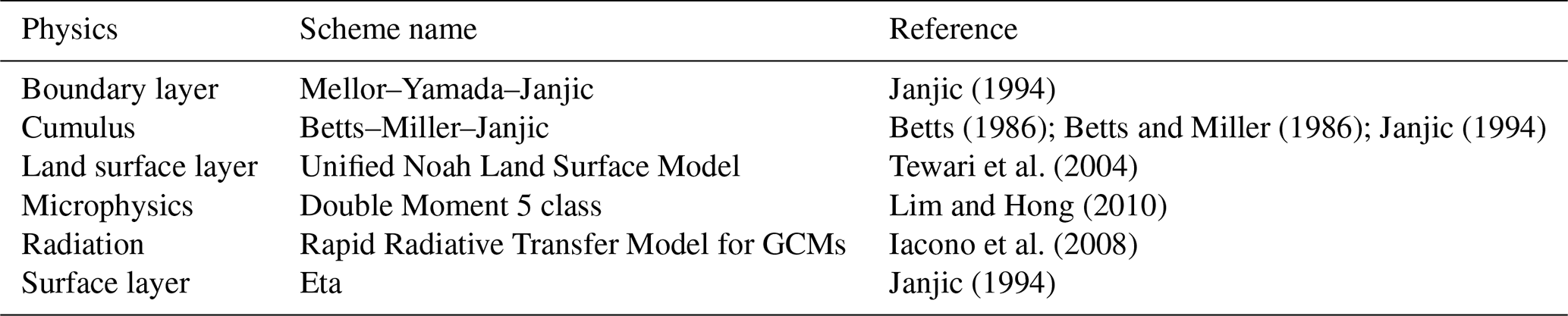
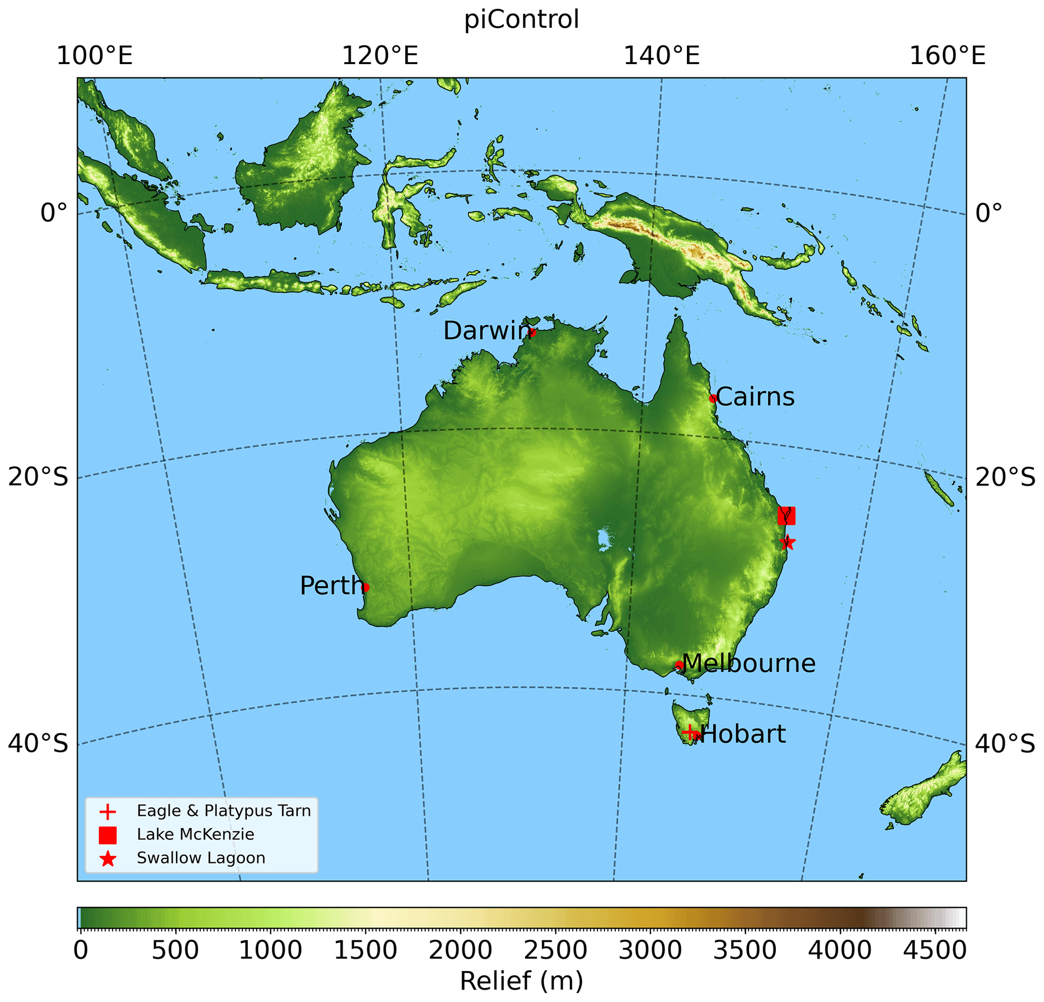
Figure 2 The topographical height from ETOPO1 for the WRF model domain. Cities and specific proxy sites mentioned in the text are shown.

Figure 3 Vegetation distribution used in the WRF simulations for pre-industrial (a) and mid-Holocene (b). See Table S1 for a description of the codes.

2.3 Proxy data

The model simulations were evaluated against a new pollen-based reconstruction of seasonal temperature, mean annual precipitation, and moisture availability (Herbert and Harrison, 2016). This data set was developed to fill the gap in the widely used pollen-based reconstruction from Bartlein et al. (2011), which has no data points in Australia. The original pollen reconstruction from Herbert and Harrison (2016) has been updated to include many more data locations (Annika Herbert, personal communication, 2020), with 239 in total. Unfortunately, due to high correlations between mean annual temperature and the two seasonal temperature variables in the modern climate, it was not possible to include all three temperature variables, and Herbert and Harrison (2016) have only provided reconstructions for the following variables: mean temperature of the warm month (MTWA), mean temperature of the cold month (MTCO), mean annual precipitation (MAP), and the plant-available moisture index (α). In addition to this continental-scale proxy data set, there are four individual sites that have been quantifiably analysed: Eagle Tarn (42.6799° S, 146.5914° E) and Platypus Tarn (42.6734° S, 146.5868° E) in Tasmania (Rees and Cwynar, 2010); Lake McKenzie (Boorangoora) (25.4475° S, 153.0533° E) on K'gari (Fraser Island), Queensland (Woltering et al., 2014); and Swallow Lagoon (27.4986° S, 153.4547° E) on Stradbroke Island (Minjerribah), Queensland (Barr et al., 2019). The two sites in Tasmania show that temperatures for the warm month in the MH were slightly cooler than present-day temperatures (Fig. 5 in Rees and Cwynar, 2010). In contrast, the MAT on K'gari (Fraser Island) in Queensland showed that temperatures were 0.9 °C warmer at 5.8±0.3 ka relative to 1950 (Woltering et al., 2014). On Stradbroke Island (Minjerribah) in Queensland, the MAP was higher by around 500 mm yr⁻¹ during the MH and much less variable than late Holocene and present-day conditions (Barr et al., 2019).

3 Results

The results of the WRF simulations are first validated against present-day conditions, followed by a discussion of the mean state of the PI and MH simulations and the differences between them. Where possible, the climate anomalies are compared to available proxy data and are re-gridded to a common rectilinear grid for analysis. Climate models use a modern calendar for monthly analysis, but the length of each month changes as the transit speed of the Earth's orbit varies with the timing of perihelion. Sub-annual model results were adjusted for the variations in these month lengths using the PaleoCalAdjust tool developed by Bartlein and Shafer (2019).

3.1 Pre-industrial climate conditions

The results of the PI simulation were validated against present-day reanalysis and satellite products. These comparisons were complicated by the differences between 1850 and late 21st century conditions but nevertheless provide a basic benchmark for the WRF simulations. To validate the MAT from the PI simulation, we obtained the ANUCLIM data set which provides monthly temperature data on a 0.05° grid over continental Australia (Xu and Hutchinson, 2011). After re-gridding the WRF and ANUCLIM data to a rectilinear 0.45° grid, the RMSE between the WRF PI simulation and ANUCLIM data was 0.29 °C (Fig. S1 in the Supplement). The temperature distribution was very similar between the PI simulation and ANUCLIM, with annual temperatures in the tropical north of Australia 27.6 °C at Darwin and 22.2 °C at Cairns, transitioning to cooler conditions in the south, 18.1 °C at Perth, 13.8 °C at Melbourne, and 11.0 °C at Hobart (Fig. 4a). There were small differences between the WRF (Fig. 4a) and CESM (Fig. S2) temperature distributions, particularly over steep topography. Validation of the precipitation was done with reference to the Tropical Rainfall Measuring Mission (TRMM) satellite data set (Huffman et al., 2010). The TRMM and WRF MAP data were re-gridded to the same rectilinear 0.45° grid, and the RMSE between the two was 0.5 m yr⁻¹ (Fig. S3). The differences between WRF and TRMM were heterogeneous (Fig. S3), with WRF simulating heavier precipitation in tropical locations over water but generally lighter precipitation over tropical land. Over mid-latitude continental Australia, WRF simulated lighter precipitation over the coastal locations south of Perth but over most of the remaining continental land WRF simulated heavier precipitation. The differences between the CESM simulation and TRMM were much larger compared to the WRF simulation. The largest values of MAP occurred in the tropics, which in the CESM simulation were up to 3.7 m yr⁻¹ (Fig. S4b), compared to 6.1 m yr⁻¹ in TRMM (Fig. S3). The annual precipitation was 1233 mm yr⁻¹ at Darwin, 772 mm yr⁻¹ at Cairns, 480 mm yr⁻¹ at Perth, 877 mm yr⁻¹ at Melbourne, and 659 mm yr⁻¹ at Hobart. Overall, the spatial distribution of the precipitation was well captured with the meridional gradient from the tropics to the Southern Ocean in the TRMM data set replicated in the WRF simulation. These small differences between WRF and the reanalysis and satellite data sets indicate that WRF is suitable for Australian palaeoclimate simulations.

Figure 4 The 2 m temperature values for the WRF pre-industrial simulation (a), mid-Holocene simulation (b), and the difference (mid-Holocene minus pre-industrial) (the significant changes, two-sided Student's t test, and 95 % confidence interval are indicated by dots) (c). The purple line in panels (b) and (c) is the coastline in the mid-Holocene.

3.2 Mid-Holocene climate conditions

The simulated MAT in the MH shows that conditions were generally very similar to PI over the Australian domain (Fig. 4). The positioning of the MAT isotherms in the MH and PI simulations is nearly identical between the two simulations (Fig. 4a, b). Compared to the PI, the MH MAT was within ±0.25 °C over most of continental Australia and in the north-west of the model domain over Borneo, Sumatra, and Java. Over the north of Australia and into the tropical seas to the north and north-east of the Australian continent, temperatures were between 0.25–1 °C warmer in the MH. The standard deviation of the MAT is predominantly below 1 °C over most of the domain, with a small area in the Kimberley and Pilbara getting up to 1.3 °C (Fig. S5a). During the MH, the MAT at Darwin was 28.2 °C, 22.4 °C at Cairns, 18.0 °C at Perth, 13.8 °C at Melbourne, and 11.0 °C at Hobart.

Figure 5 Seasonal 2 m temperature differences between the mid-Holocene and pre-industrial period for MTWA (a, c, e) and MTCO (b, d, f). The top row is the WRF simulations in panels (a) and (b). The middle row is the CESM simulations in panels (c) and (d). The bottom row is the pollen proxy data set (Herbert and Harrison, 2016) at 2° resolution in panels (e) and (f). In panels (a), (b), (c), and (d) the purple line is the coastline in the mid-Holocene, and significant changes, the two-sided Student's t test, and 95 % confidence interval are indicated by dots.

The January temperatures over the Australian continent were predominantly cooler during the MH, on average 0.35 °C cooler over Australia (Fig. 5a) and were mostly statistically significant at the 95 % level, and during July in the north-west of Australia, temperatures were slightly warmer, with a continental average of 0.19 °C warmer (Fig. 5b). These continental conditions were in response to the positive insolation anomalies in the austral winter and early spring and negative anomalies in the austral summer and autumn (Fig. 1). There was, however, a large range of year-to-year fluctuations in seasonal temperatures over continental Australia in both the MH and PI, such that on any given year, conditions could have been warmer or cooler in the MH relative to the PI (Fig. S5c, d). The oceanic response to insolation, however, was the opposite, with warmer tropical and Southern Ocean conditions in January. The warmer conditions over tropical Australia and into the Maritime Continent in January match the response from the coarser-resolution ESM, where temperatures over the tropical latitudes were 0.25–1 °C warmer in the MH (Fig. 5c). The oceanic response reflects the higher inertia of water relative to land that mutes the temperature response due to the changing insolation forcing during the austral summer.

The proxy evidence for MH temperatures showed a cooling trend for both January and July (Fig. 5e, f); in a few locations, these were significantly cooler, particularly in tropical latitudes. Over south-eastern Australia, the proxy evidence indicates that temperatures were both cooler and warmer, depending on the grid cell. In January, temperature differences were larger than in July, but there was an unclear picture that the MH was generally cooler or warmer, as the results appear to be specific to the location of the proxy record. The mean absolute error (MAE) between the proxy evidence and the two simulations was very similar at 2° resolution for both MTWA and MTCO, with 2.8 and 2.7 °C respectively (Tables S2 and S3). If, however, the proxy and WRF results are re-gridded at 0.45° resolution, then the MTWA reduces to 2.4 °C, which is an improvement relative to the coarser-scale CESM result.

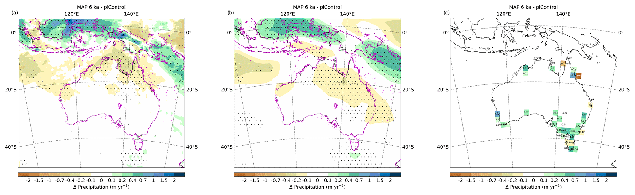
Figure 6 Annual precipitation differences between the mid-Holocene and pre-industrial period from the WRF simulations (a), the CESM simulations (b), and pollen-based proxy data from Herbert and Harrison (2016) at 2° resolution (c). In panels (a) and (b), significant changes, the two-sided Student's t test, and 95 % confidence interval are indicated by dots, and the purple line is the coastline in the mid-Holocene.

Annual precipitation during the MH was within ±0.1 m yr⁻¹ of the PI over most of continental Australia and particularly south of 20° S (Fig. 6a). Over the tropical latitudes, the MAP was more heterogeneous, with drier conditions over northern Australia and the north-east Indian Ocean but wetter conditions over the equatorial islands of the Maritime Continent and the Solomon Sea. The same pattern exists in the tropics in the coarser-resolution CESM results (Fig. 6b), although the magnitude of the responses was more muted, particularly over the equatorial latitudes. The WRF model at the finer resolution captured the orographic effects at these locations, particularly over New Guinea. The wetter anomalies over the equatorial Maritime Continent, Solomon Sea, and the highlands of New Guinea were statistically significant at the 95 % level, stemming from the smaller relative year-to-year fluctuations at these locations (Fig. S5b). The same is true of the drier anomalies in the Arafura Sea and the Gulf of Carpentaria, where the year-to-year fluctuations were much smaller. In the north-east Indian Ocean and equatorial western Pacific Ocean, the anomalies were not statistically significant at the 95 % level, due to the large fluctuations in year-to-year precipitation differences (Fig. S5b). The MAP during the MH was 1023 mm yr⁻¹ at Darwin, 546 mm yr⁻¹ at Cairns, 442 mm yr⁻¹ at Perth, 873 mm yr⁻¹ at Melbourne, and 698 mm yr⁻¹ at Hobart.

The proxy evidence for MH precipitation showed a generally wetter continent, except for a few individual locations. In south-east Australia, where most of the proxy data exist, precipitation was predominantly heavier in the MH up to 700 mm yr⁻¹, which would constitute a near-doubling of precipitation from modern conditions. Over Cape York Peninsula, the proxy data showed both a wetter and drier climate during the MH, depending on the sample location. The MAE between the proxy evidence and CESM was 352 mm yr⁻¹, compared to 363 mm yr⁻¹ for WRF at 2° resolution (Table S4). Re-gridding the proxy and WRF results to 0.45° reduced the MAE to 294 mm yr⁻¹, which is a 20 % improvement.

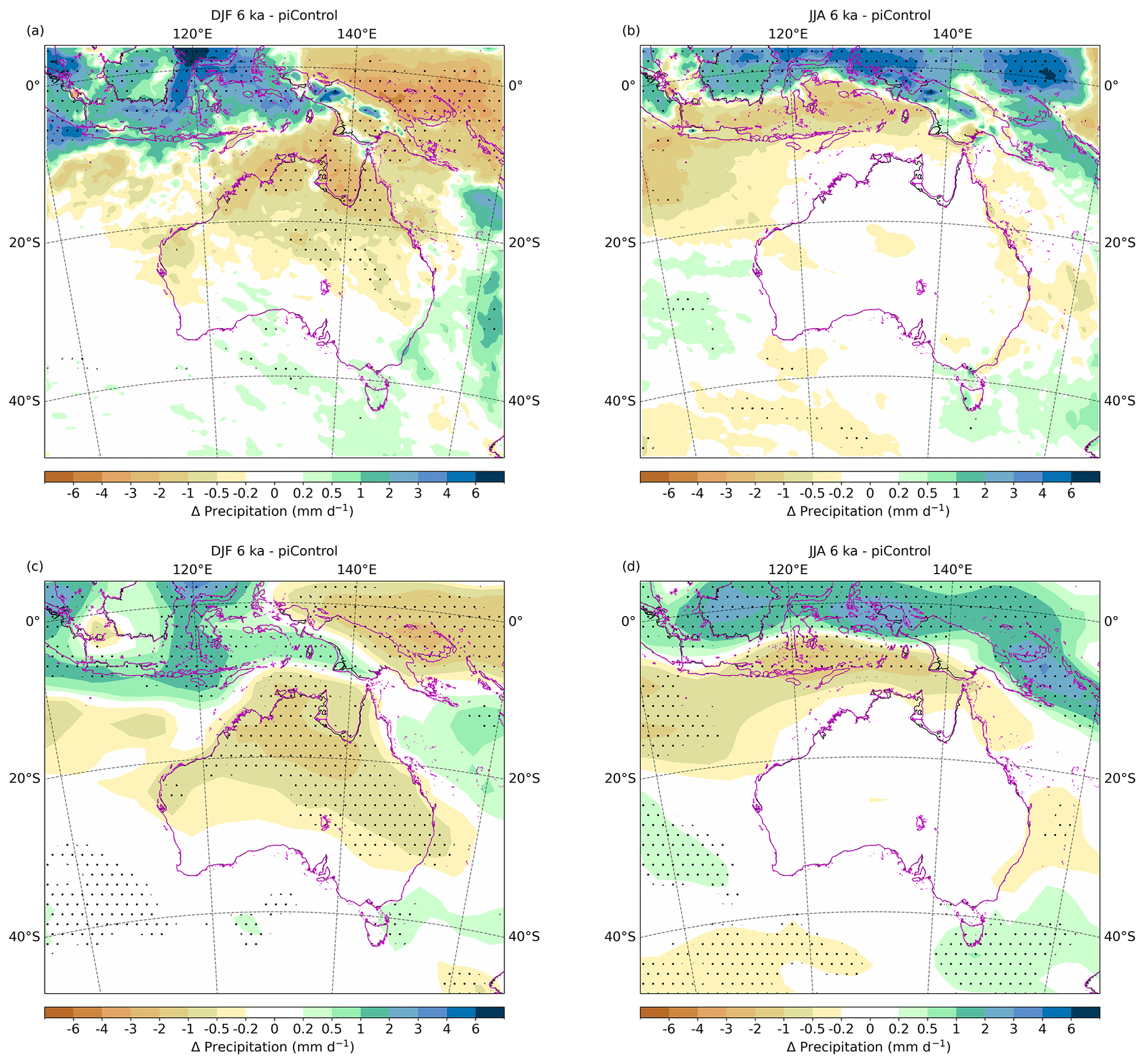
Figure 7 Seasonal precipitation differences between the mid-Holocene and pre-industrial period for December, January, and February from the WRF simulations (a); June, July, and August from the WRF simulations (b); December, January, and February from the CESM simulations (c); and June, July, and August from the CESM simulations (d). Significant changes, the two-sided Student's t test, and 95 % confidence interval are indicated by dots, and the purple line is the coastline in the mid-Holocene. Note the different units compared to Fig. 6.

During the austral summer, precipitation over most of continental Australia was less during the MH, extending into the Timor and Arafura seas and over most of New Guinea and into the equatorial western Pacific Ocean (Fig. 7a, c). The dry anomalies over New South Wales, the southern Northern Territory, and Queensland were statistically significant at the 95 % level, but the year-to-year fluctuation was much larger in the north-west of the domain (Fig. S6a). Across the Indonesian archipelago, precipitation conditions were much wetter during the MH but only statistically significant at the 95 % level in locations of the largest anomalies. This summertime precipitation over the Indonesian–Australian monsoon region indicates a sharp north-west–south-east transition between the MH and PI. There was a strong intensification in the north-western part of the monsoon tropics, which transitioned to drier conditions in the south-eastern part of this domain. The WRF model at the finer resolution was able to simulate much larger precipitation rates, which are illustrated in the differences in the magnitude of the anomaly in the summertime precipitation (Fig. 7a, c).

The seasonal wind anomalies, along with sea level pressure (SLP), are shown in Fig. 8. Summertime SLP was reduced in the MH over most of the domain, except in the centre of continental Australia and in the south of the domain (Fig. 8a). There was reduced westerly flow during the MH over the Indonesian archipelago, indicating weaker monsoon conditions relative to PI (Fig. 8a), which was coincident with reduced summertime precipitation (Fig. 7a, c). This was also evident in the 850 hPa zonal wind anomalies between 15° S and the Equator (Fig. S8c). Over the tropical latitudes, the precipitation anomalies were coincident with vertically integrated water vapour convergence (VIWVC) anomalies (Fig. 9a), indicating local dynamical processes. The size of the monsoon convergence zone was slightly enlarged in the MH (Fig. S7a) compared to PI (Fig. S7b), although the southern extent was similar just south of 20° S. This increased convergence zone differs over northern Arnhem Land, which contributed to the reduced precipitation there from weaker westerly flow. In the extra-tropics, there was also reduced westerly flow over the Southern Ocean in the MH summertime relative to PI (Fig. 8a), coincident with increased summertime temperatures (Fig. 5a, c) but not coincident with a decline in precipitation (Fig. 7a, c).

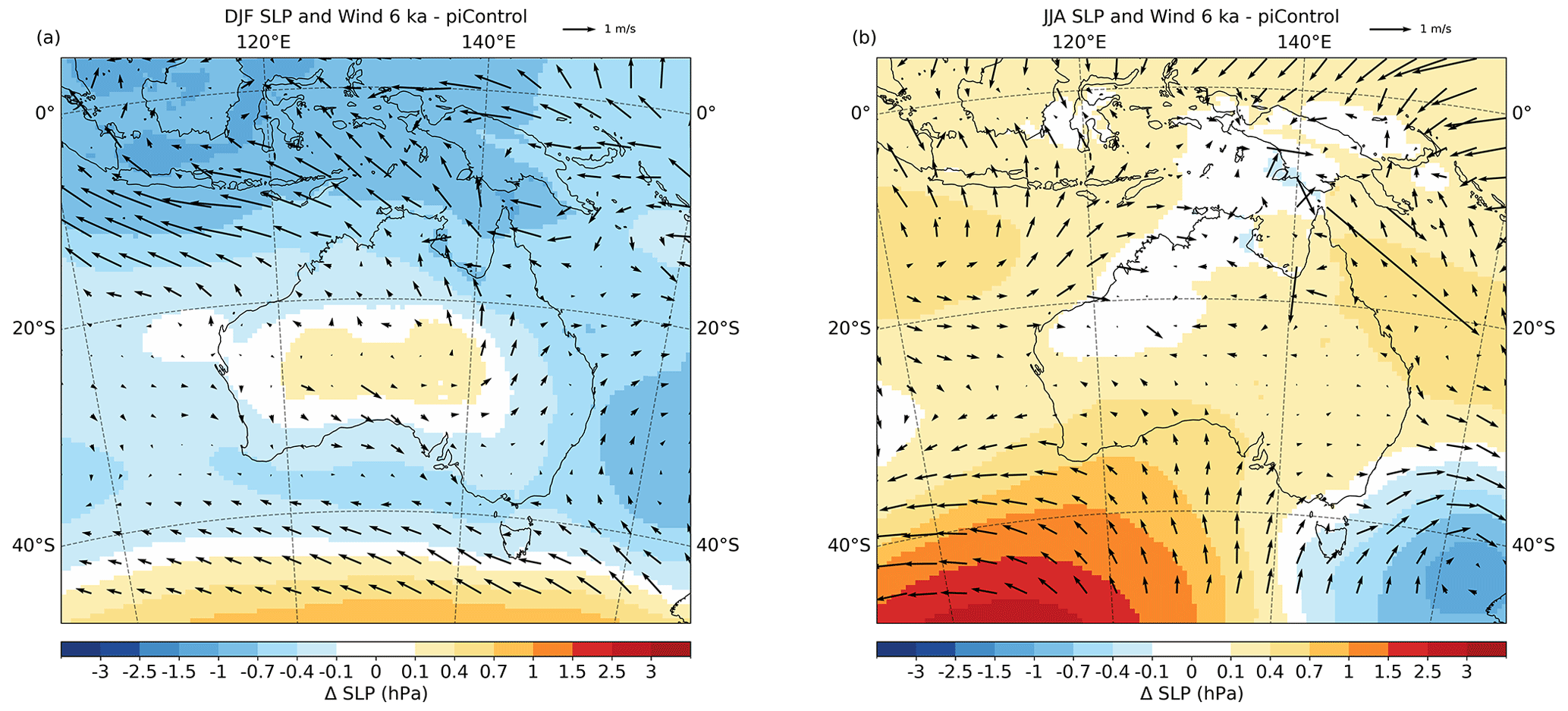
Figure 8 Sea level pressure (SLP) as the coloured contours and wind speed as the vectors of the differences between the mid-Holocene and pre-industrial period from the WRF simulations for December, January, and February (a) and June, July, and August (b).

During the austral winter, precipitation differences were almost entirely within ±0.2 mm d⁻¹ over continental Australia (Fig. 7b, d), although there was a large year-to-year fluctuation of up to 2 mm d⁻¹ (Fig. S6b). Over the north-eastern Indian Ocean and across the Indonesian archipelago into the Java and Banda seas, conditions were drier by up to 2 mm d⁻¹. Across the Equator in Borneo, the Celebes Sea, and over New Guinea, precipitation was much heavier during the MH. Similar to the continental results, there were large year-to-year fluctuations. The only locations where the anomalies were statistically significant (at the 95 % level) were the positive anomalies in the tropics and a few scattered oceanic locations in the west and south of the domain (Fig. 7b).

The relationship between wintertime precipitation and SLP or wind anomalies was less clear than in summertime. Wintertime SLP was predominantly higher in the MH (Fig. 8b), but there was a region of increased SLP over the southern Tasman Sea and increased westerly flow which was coincident with increased precipitation (Fig. 7b, d). In the Southern Ocean to the south of Australia, there was increased SLP and weaker westerly flow, which was coincident with reduced precipitation (Fig. 7b, d). The convergence zone between the south-easterly trades and extra-tropical westerlies was located at a similar latitude in both the MH and PI simulations at around 30° S (Fig. S7c, d), and there was a negligible difference in the zonally averaged 850 hPa extra-tropical westerlies (Fig. S8d). The tropical precipitation anomalies were coincident with locations of VIWVC (Fig. 9b).

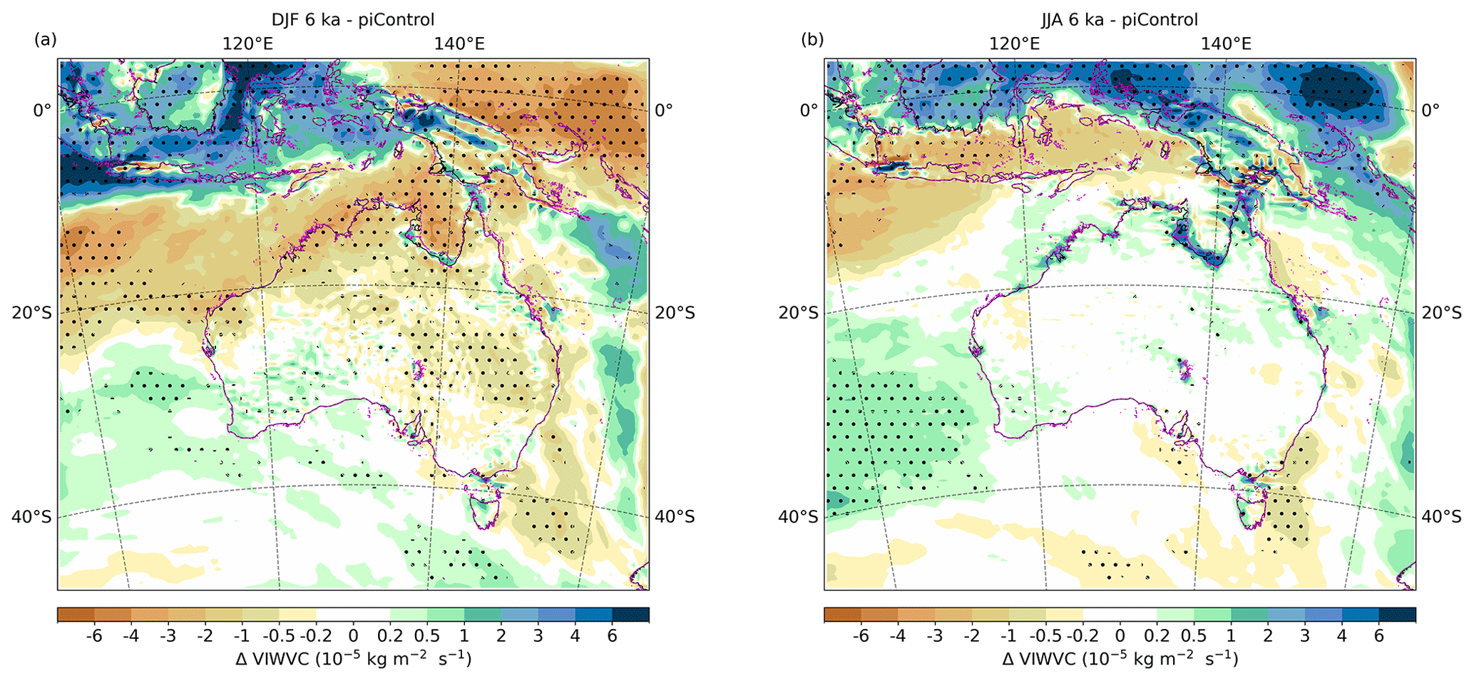
Figure 9 Vertically integrated water vapour convergence differences between the mid-Holocene and pre-industrial period from the WRF simulations for December, January, and February (a) and June, July, and August (b). Significant changes, the two-sided Student's t test, and 95 % confidence interval are indicated by dots, and the purple line is the coastline in the mid-Holocene.

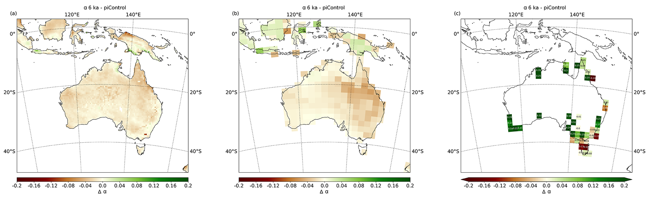
Figure 10 Mean annual plant-available water index (α) differences between the mid-Holocene and pre-industrial period from the WRF simulations (a), the CESM simulations (b), and pollen proxy data (c). The model results in panels (a) and (b) are masked for cells, where ≥ 25 % of the cell is land.

The moisture availability index (α) is the ratio of actual evapotranspiration to equilibrium evapotranspiration on an annual basis and can indicate the amount of growth-limiting drought stress on plants (Prentice et al., 1993). In both the WRF and CESM simulations, α was slightly lower during the MH over continental Australia. In the WRF simulation, there was a small region of positive anomalies in western Carpentaria which was the location of the warmest MAT differences (Fig. 4c). In the tropics to the north of Australia, there were two locations of positive α anomalies in the WRF simulation, on Java and southern New Guinea, which coincided with locations of increased precipitation (Fig. 6a). In contrast to this, however, in the north of New Guinea there was a location with large decreased α, where precipitation was also increased during the MH. The CESM simulation indicates positive α anomalies in the MH in the tropics to the north of Australia, which is in contrast to the WRF simulation (Fig. 10b). The α differences between CESM and WRF in the tropics were related to decreases in the equilibrium evapotranspiration during the MH in the CESM simulation. These tropical locations were also regions of the largest precipitation values (Fig. S4), and the WRF simulation replicated the magnitude of annual precipitation that was closer to the TRMM data set (Fig. S3). The locations of these higher α differences are associated with smaller precipitation anomalies in the CESM simulations, and these are co-located with slightly increased evapotranspiration.

The lower α anomalies over continental Australia contrast with most of the proxy evidence (Fig. 10c), which shows mostly positive anomalies, although there were some grid cells in south-eastern Australia that show negative anomalies. The MAE between the proxy data and CESM simulation was 0.11, which was higher than the WRF simulation at 0.08 at 2° resolution and improves when the proxy data are compared to the WRF simulation at 0.45° resolution with a MAE of 0.06 (Table S5).

4 Discussion

The previous section outlined the changes in climate over the Australian region at the MH compared with PI conditions from the coarser-resolution simulation of CESM and the finer-resolution simulation of WRF and how these two simulations compared with results from bioclimate modelling using proxy evidence. This section will summarise these findings and compare them to other work.

4.1 Temperature

The MAT in both CESM and WRF were largely in agreement, showing statistically significant warming of 0.25–1 °C over central Australia into the northern tropics and extending into the seas between Indonesia, New Guinea, and Australia (Fig. 4c). These warmer temperatures contrast with the multi-member ensemble of PMIP3 and PMIP4 anomalies for the MH that found a 0–0.3 °C cooling over continental Australia (Brierley et al., 2020) and a 0.25–0.5 °C cooling from CESM2 (Otto-Bliesner et al., 2020). The spread of results from the multi-member ensemble (Brierley et al., 2020) suggests that some models simulated warming over Australia, but this would still predominantly fall below the results presented here. Despite this, the qualitative summary from the OZ-INTIMATE project found that there was a thermal expansion of the Indo-Pacific Warm Pool (IPWP) during the MH (Reeves et al., 2013b), which would agree with the temperatures found in Fig. 4c. The one annual temperature record from the proxy literature found that the temperature on K'gari (Fraser Island) was 0.9 °C warmer in the MH (Woltering et al., 2014), which was above that found in either CESM (not shown) or WRF (Fig. 4c).

The austral winter temperatures in Australia were warmer or the same in the MH, with a few coastal and oceanic locations showing slightly cooler temperatures in both the CESM and WRF simulations (Fig. 5). The CESM simulation found that the warmer winter temperatures traversed the width of the continent, whereas in the WRF simulation, the warmer temperatures were only in the central and north-west of Australia. WRF also simulated cooling over Tasmania and the Gulf of Carpentaria that was not found in the CESM simulation. The multi-member ensemble of PMIP3 and PMIP4 simulations found a warming over continental Australia (Brierley et al., 2020), which was in agreement with the CESM simulation and mostly in agreement with the WRF simulation. The CESM2 simulation found winter temperatures were ±0.25 °C over continental Australia (Otto-Bliesner et al., 2020). Over oceanic grid cells, the PMIP3 and PMIP4 simulations were cooler during the MH, which contrasts with the CESM and WRF simulations. The spread of results in the multi-member ensemble (Brierley et al., 2020) suggests that some models simulated conditions found in the CESM and WRF simulations.

The austral summer temperatures in Australia were cooler over the sub-tropical and mid-latitude locations in the WRF simulation and in a slightly less uniform manner in the CESM simulation (Fig. 5). In the tropics and to the south of continental Australia, temperatures were warmer in the MH. Over continental Australia, a similar result was found in the multi-member ensemble from PMIP3 and PMIP4 results, with a cooling of 0.3–1.2 °C (Brierley et al., 2020). Over oceanic grid cells, the multi-member ensemble found summer temperatures were cooler in the MH by 0–0.3 °C relative to PI (Brierley et al., 2020), which contrasts with the tropical and Southern Ocean results found in both the CESM and WRF simulations. The WRF and CESM results were more closely aligned with the CESM2 simulation from Otto-Bliesner et al. (2020), who found cooler land temperatures, but the tropical and mid-latitude ocean temperatures were ±0.25 °C. There were two proxy records for warm month MH anomalies from Tasmania, both showing that conditions were slightly cooler during the MH (Fig. 5 in Rees and Cwynar, 2010), which contrasts with the warmer temperatures found in both the CESM and WRF simulations.

The MH temperatures from the pollen proxy data set showed a cooling in the MH over northern Australia in the austral winter and summer (Fig. 5e, f). Over the southern latitudes of Australia, the proxy records show some locations with cooling in the MH and warming in others, depending on the exact grid cell; these results exist in both the warm and cold months. The temperature anomalies shown in Fig. 5e and f were re-gridded to 2°, but the extreme values exist at higher resolutions as well. There are multiple potential causes of these extreme values discussed in Herbert and Harrison (2016). The first is that to improve the number of sites included in the data set, surface conditions from a gridded data set (i.e. ANUCLIM) were used for all sites and not core tops, as not all sites have a core-top value. The justification for this was that this increased the number of sites that can be included in the data set, which outweighed the use of sites with only core-top values (Herbert and Harrison, 2016). The downside was that site-specific information was lost from the core top, which would reduce some of the extreme cases. A second contributing factor was when there was pollen identified that has a few modern analogues; this can lead to large biases in the results. Despite these concerns, the data set is a valuable reference from which modelling results can be compared. The results presented here show that there was an improvement in using the finer-resolution results for the modelling of warm month anomalies compared to the coarser results from CESM. The same was not evident in the cold month results, but there was nevertheless no detriment in the model–proxy comparison, and the increased resolution facilitates the identification of some fine-scale effects in coastal and locations of steep orography that are not captured in the coarser model results.

4.2 Precipitation and moisture

The MAP during the MH was slightly reduced over tropical latitudes of continental Australia in the WRF simulation and in the north and east of Australia in CESM (Fig. 6a, b). Over the remainder of Australia, precipitation was the same during the MH and PI. In the equatorial tropics, annual precipitation was heavier over Borneo, New Guinea, and the islands of the Banda Arc. To the immediate north of Australia, precipitation was reduced in the MH, which extended onto the north of the continent in the WRF simulation. There was one site on Stradbroke Island (Minjerribah) in Queensland that found that the MAP was higher by around 500 mm yr⁻¹ during the MH (Barr et al., 2019), which was a result not replicated in the WRF or CESM simulations. The bioclimatic evidence from the OZ-INTIMATE series found that river discharge was enhanced in temperate climates (Petherick et al., 2013) but that conditions were more arid in the interior of the continent (Fitzsimmons et al., 2013). In the Australian tropics, there was a reduction in the fluvial activity and re-activation of dunes in Lake Gregory in north-western Australia (Reeves et al., 2013b), with mangrove contraction from 7.4 ka (Proske et al., 2014) and reductions in rainforest taxa (Field et al., 2017) in the Kimberley. There was a slight equatorward shift in the Intertropical Convergence Zone and contraction of the extent of the IPWP, resulting in a small reduction in monsoon activity over northern Australia (Reeves et al., 2013b). These reductions in the northern Australian precipitation agree with the findings in the WRF and CESM simulations.

To provide a more quantifiable analysis between the modelling and the bioclimatic results, the simulations were compared to the pollen proxy data set. The pollen proxy data set also found precipitation was generally increased in the MH (Fig. 6c), except for a couple of locations around Cape York Peninsula and the east and south-east of Australia. The bias between the proxy data set and the simulations was similar at 2° but improved by 20 % for the WRF simulation when the resolution was reduced to 0.45°. The moisture availability variable (α) also had a reduction in the bias in the WRF simulation compared to the CESM. These results highlight the benefit of finer-resolution models over and above the better representation of changes in response to feedback and physical processes.

On a seasonal basis, the austral winter precipitation was similar between MH and PI over continental Australia. The largest differences were evident in the intensification of equatorial precipitation, contrasting with a reduction over the Java Sea, Banda Sea, and the north-east Indian Ocean. The same differences in tropical wintertime precipitation were found in the CESM2 simulation from Otto-Bliesner et al. (2020) and the multi-model ensemble of PMIP3 and PMIP4 simulations (Brierley et al., 2020). The overall wintertime precipitation distribution for the whole domain matches that from CESM2 and the multi-model ensemble.

The summertime precipitation is dominated by the Indonesian–Australian monsoon, although the level of dryness in the south of Australia can influence drought and forest fires. The summertime precipitation in the higher latitudes of Australia was very similar between MH and PI, although the WRF simulation found slightly wetter conditions over Tasmania and eastern Victoria. In the tropical north of Australia, summertime precipitation was reduced in the MH in both the CESM and WRF simulations as far north as the Indonesian archipelago. A similar trend was found in the multi-member ensemble, although the reduction in precipitation was more severe, up to 0.8 mm d⁻¹ (Brierley et al., 2020). The CESM2 simulation showed that only continental Australian grid cells experienced reductions at the MH, which transitioned to increased precipitation in the Timor and Arafura seas (Otto-Bliesner et al., 2020). The reductions in summertime precipitation were considered to be a result of a response to the timing of the perihelion, which shifted to the austral spring equinox during the MH and resulted in a northward propagation of the summertime precipitation domain (Brierley et al., 2020; Jiang et al., 2015). In a different multi-model analysis focussing on the mid-Holocene Southern Hemisphere monsoon, D'Agostino et al. (2020) found that the northern Australian monsoon extent over land grid cells contracted 13.8 %, and the precipitation was 10.5 % lower in the MH. D'Agostino et al. (2020) used the moisture budget decomposition to show that the reductions in MH monsoon activity were primarily dynamical weakening, i.e. stronger anticyclonic conditions and a westward shift in the main Walker circulation updraught. The WRF simulation showed a similar weakening of westerly winds over the north-eastern Indian Ocean and slightly increased SLP over the middle of the continent (Fig. 8a), which reduced the onshore flow on the western coastline of tropical Australia and caused the resultant decrease in summertime precipitation.

5 Conclusions

This research presents the first evaluation of downscaled climate modelling of the MH climate over Australia and the surrounding region. This evaluation consisted of simulating the MH and PI climate, with an ESM and RCM, and analysing both simulations against the available proxy records. These results offer the highest-resolution analysis of the MH climate over Australia. The model results show that there was little difference in temperature over southern Australia between the MH and PI, and over northern Australia and into the tropics, temperatures were slightly warmer during the MH relative to PI. Precipitation during the MH was generally reduced over northern Australia and in the Indonesian–Australian monsoon region, particularly during summertime months. The results of the coarser ESM and finer RCM were generally in agreement; however, significantly greater granulation was evident in the finer-resolution WRF simulations in response to the depiction of feedback and physical processes. The comparison of the two simulations to the pollen proxy data set shows that there was some improvement to be gained from the finer-resolution model. These improvements were reductions in the MAE between the model and proxy data of the MTWA, MAP, and moisture availability index.

Further analysis is required to investigate the drivers of the changes in the monsoon by decomposing the moisture budget into its thermodynamic and dynamic components. Such an analysis will provide insights into the mechanisms that establish the Indonesian–Australian monsoon. Future analysis would also benefit from improvements in the bioclimatic proxy evidence. A greater number of sites, particularly in the arid interior, would help validate the model results, where presently the model simulations are the only data points that can provide a representation of the MH palaeoclimate.