Simulation of a former ice field with Parallel Ice Sheet Model – Snežnik study case

In this paper, we present a reconstruction of climate conditions during the Last Glacial Maximum on a karst plateau Snežnik, which lies in Dinaric Mountains (southern Slovenia) and bears evidence of glaciation. The reconstruction merges geomorphological ice limits, classified as either clear or unclear, and a computer modelling approach based on the Parallel Ice Sheet Model (PISM). Based on extensive numerical experiments where we studied the agreements between simulated and geomorphological ice extent, we propose using a combination of a high-resolution precipitation model that accounts for orographic precipitation combined with a simple elevation-based temperature model. The geomorphological ice extent can be simulated with climate to be around 6 °C colder than the modern day and with a lower-than-modern-day amount of precipitation, which matches other state-of-the art climate reconstructions for the era. The results indicate that an orographic precipitation model is essential for the accurate simulation of the study area, with moist southern winds from the nearby Adriatic Sea having a predominant effect on the precipitation patterns. Finally, this study shows that transforming climate conditions towards wetter and warmer or drier and colder does not significantly change the conditions for glacier formation.

1 Introduction

The Last Glacial Maximum (LGM) in Europe was dominated by the Fennoscandian Ice Sheet, which was one of the major global ice masses during the last glacial cycle. A relatively large ice mass was also the Alpine ice sheet over the European Alps. Other, much smaller, mountain glaciers existed in Iberia, the Pyrenees, the Apennines, and the Balkans (Hughes et al., 2013). These smaller ice masses, being isolated from larger ice sheets, have a well-defined linkage between their areas of origin and the areas they affect, which simplifies the task of reconstructing their past extents and behaviours. Additionally, their tendency to react quickly to climate change makes them valuable proxies for deducing historical climate conditions.

Past glaciations in the northern Dinaric Mountains at the interface between the Alpine ice sheet and Balkan Mountain glaciers are well-documented geomorphologically (e.g. Žebre et al., 2013, and Žebre and Stepišnik, 2016), but there is lack of knowledge about climate–glacier dynamics based on the modelling approach. The northern Velebit mountains in Croatia are the only formerly glaciated mountains in this region where an empirical reconstruction has been compared with computer-based simulations under different palaeoclimate forcings (Žebre et al., 2021). In southern Slovenia, only a few kilometres to the north of Velebit, lies Snežnik, one of the northernmost mountain plateaux in the northern Dinaric Mountains. Snežnik was glaciated during the LGM, although the exact timing is still ambiguous (Marjanac et al., 2001; Žebre et al., 2016). Moraines that mark the farthest extent of the glacier have been attributed to the LGM, for which the maximum ice area was estimated to be at least 40 km² (Žebre and Stepišnik, 2016). Although the formerly glaciated area is very small compared to the large Alpine ice sheet (estimated to be 163 000 km² by Seguinot et al., 2018), detailed knowledge of it can still aid in deciphering the regional past climate conditions. There have been only a few attempts to model the palaeo-ice field on the Snežnik mountain either only on the limited area around the small Snežnik summit (Žebre and Stepišnik, 2016) or as part of a larger Alpine area (Seguinot et al., 2018). In the first case, a simple steady-state model that assumes a perfectly plastic ice rheology was applied (Benn and Hulton, 2010), while in the second case, the Parallel Ice Sheet Model (PISM) was used (the PISM authors, 2023). However, modelling small palaeoglaciers like the one on Snežnik is challenging, especially due to the need for high-resolution climate data and proxy-based palaeoclimate forcings – but also due to insufficient knowledge of pre-ice topography and ice flow.

In this work, we focus on amending the geomorphological knowledge with a computer model focused on the whole Snežnik ice field. We aim to discover the climatological conditions required for the ice field to form to an extent that is evident from the field observations. We approach the modelling challenge using the PISM on lidar-based topography with 50 m resolution and with a standard glacier modelling approach (Bueler and Brown, 2009) and custom climate-forcing models. Near-surface air temperature and precipitation are used as climate-forcing inputs in PISM, and we have developed custom models for using the available topology, single weather station data, and the knowledge of current wind patterns in the broader area. We present and explore several climate-forcing models ranging from simple to complex. In the case of Snežnik, the main challenge is achieving ice distribution according to the geomorphological evidence, which is skewed counter-intuitively, i.e. towards the well-insolated southern slopes of the plateau. The inability of the simulations to achieve an ice cover extent skewed similarly to the estimated extent can be attributed to inaccuracies in many of the used models, including sliding laws, basal conditions, and climate forcing. In this work, we chose to only address the latter, since a plethora of climate data are available that could lead to simulation improvement if integrated into the computer models.

Through the use of orographic precipitation coupled with a simple elevation-based temperature model, we manage to simulate ice field distributions that conform better to the geomorphological evidence. We find optimal overall precipitation and temperature offsets relative to modern values to be a close match to the established estimates of local precipitation and temperature in the LGM, thus giving more evidence for these estimates. We are, however, unable to credibly simulate the finer details of the ice field, such as smaller outlet glaciers.

As a part of the study, we set up a framework for an automatic quantitative assessment of the conformance of the simulated ice area to the given geomorphologically determined ice bounds. This framework is novel in its ability to work with two types of bounds, clear and unclear, and evaluates the accuracy using two criteria. We also provide a simplification that combines these two criteria into one which can then be used as an objective within the task of optimising computer model parameters.

2 Study area

Snežnik (45°34^′53^′′ N, 14°25^′53^′′ E) is a wide karst plateau with an area of roughly 100 km² in the northern part of Dinaric Mountains in Slovenia. The highest summit is Veliki Snežnik (1796 m a.s.l.).

2.1 Glacial geomorphology

Geomorphology of the area has been studied well, with studies realising the ice extent appearing as early as 1959 (Šifer, 1959). More recent works largely confirmed the previous findings (Žebre and Stepišnik, 2016) but also focused on detailed geomorphology, geochronology, and glacial–karst interaction (Žebre et al., 2016, 2019). These found that most glacial deposits are present between 900 and 1200 m a.s.l. They form characteristic glacial depositional features which stand out from the surrounding karstic area, whereas typical glacial erosional features are not common for the area. Instead, the area is dissected by glaciokarst depressions which are most likely formed by a combination of karst processes and subglacial erosion, e.g., as described in Smart (1987); Žebre and Stepišnik (2016). The maximum geomorphological ice extent in Snežnik was estimated, based on the overall position of glacial features, and which was subsequently divided into clear and unclear ice boundaries. The first were delineated based on end-moraines and outwash fans, while the latter were drawn over areas that only show suggestive evidence for glaciation. The geochronological data (Marjanac et al., 2001; Žebre et al., 2019), although still scarce, point to a maximum ice extent during the last glacial maximum (LGM), i.e. 30–17 ka (Lambeck et al., 2014).

Southeast of Snežnik lies the Gorski Kotar mountain range, which was also glaciated. Geomorphological mapping suggests that the Gorski Kotar ice field was approximately twice as large as that of Snežnik (Žebre and Stepišnik, 2016). Despite the close proximity of the two areas, there is no evidence to suggest that the two ice fields were connected (Žebre et al., 2016). Because of that and for computational reasons, the Gorski Kotar area was not included in our modelling domain.

2.2 Climate

Plateau declines to the south and the southwest towards the Adriatic Sea that starts around 25 km away. With the proximity of Adriatic Sea, the plateau is provided with above-average precipitation for the area. Snežnik receives between 2000 and 3000 mm of precipitation annually, with a strong annual cycle, as reported by ARSO (2023). There are two major drivers of precipitation, namely the Genoa low cyclone and the regular moist wind blowing from the south–southeast, which are intensified by the orographic topology. The mean annual air temperature at the meteorological station in Mašun (period 1971–1986), NW of Snežnik, is around 7 °C and average air temperatures for winter and summer are −3 and 15 °C, respectively. The rise in the specified temperatures at Mašun, relative to the pre-industrial era, can be estimated from the average of Slovenia published by Urad za meteorologijo, hidrologijo in oceanografijo (2021) and is 0.4 °C relative to pre-industrial era. Global temperature at the LGM was 3 to 6 °C lower than in pre-industrial times (Annan and Hargreaves, 2013), whereas the LGM temperature offset over the Alps has been recently simulated to about −6.6 °C (Del Gobbo et al., 2023). As for the precipitation in the LGM, the same research suggests the Alps were overall drier (by ≈ 16 %) than in pre-industrial times. Del Gobbo et al. (2023) found a similar LGM temperature and precipitation offset for the northern Dinaric Mountains in general but allowed up to ≈ 30 % drier climate around Snežnik. (Fig. 3 in Del Gobbo et al., 2023). During the last glacial cycle, the sea level in the Adriatic was 100–130 m lower than at present (Spratt and Lisiecki, 2016; Gowan et al., 2021), positioning Snežnik much further from the coastline, and associated moisture source, at a distance of 150–200 km.

3 Methods

3.1 PISM setup

PISM 2.0 was used throughout the experiments. The modelling parameters of PISM were set identically to those described in Žebre et al. (2021), where a larger mountain range just to the south of Snežnik was simulated, and similar to those in (Candaş et al., 2020), where a similarly sized mountain in the Republic of Türkiye was simulated. In this section, we list all the parameters that require an explicit setting, along with some of those that were left at their default values but were being analysed in preliminary testing and sensitivity analysis. Model selection is listed first in Table 1, and the parameters that either depend on the model selection or are general are listed in Table 2. Finally, the various settings that do not translate to PISM parameters directly are listed in Table 3.

Table 1 PISM models used in the study.

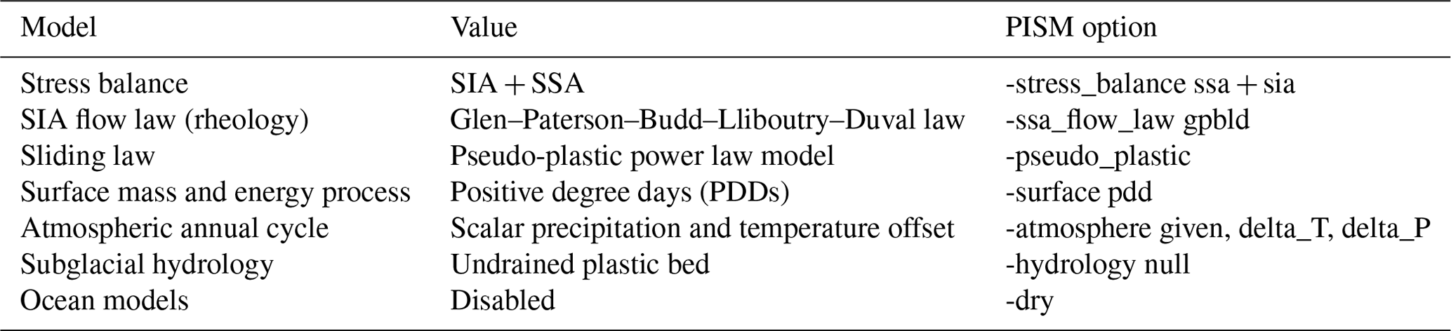
Table 2 PISM parameters that do not depend on the domain size and resolution.

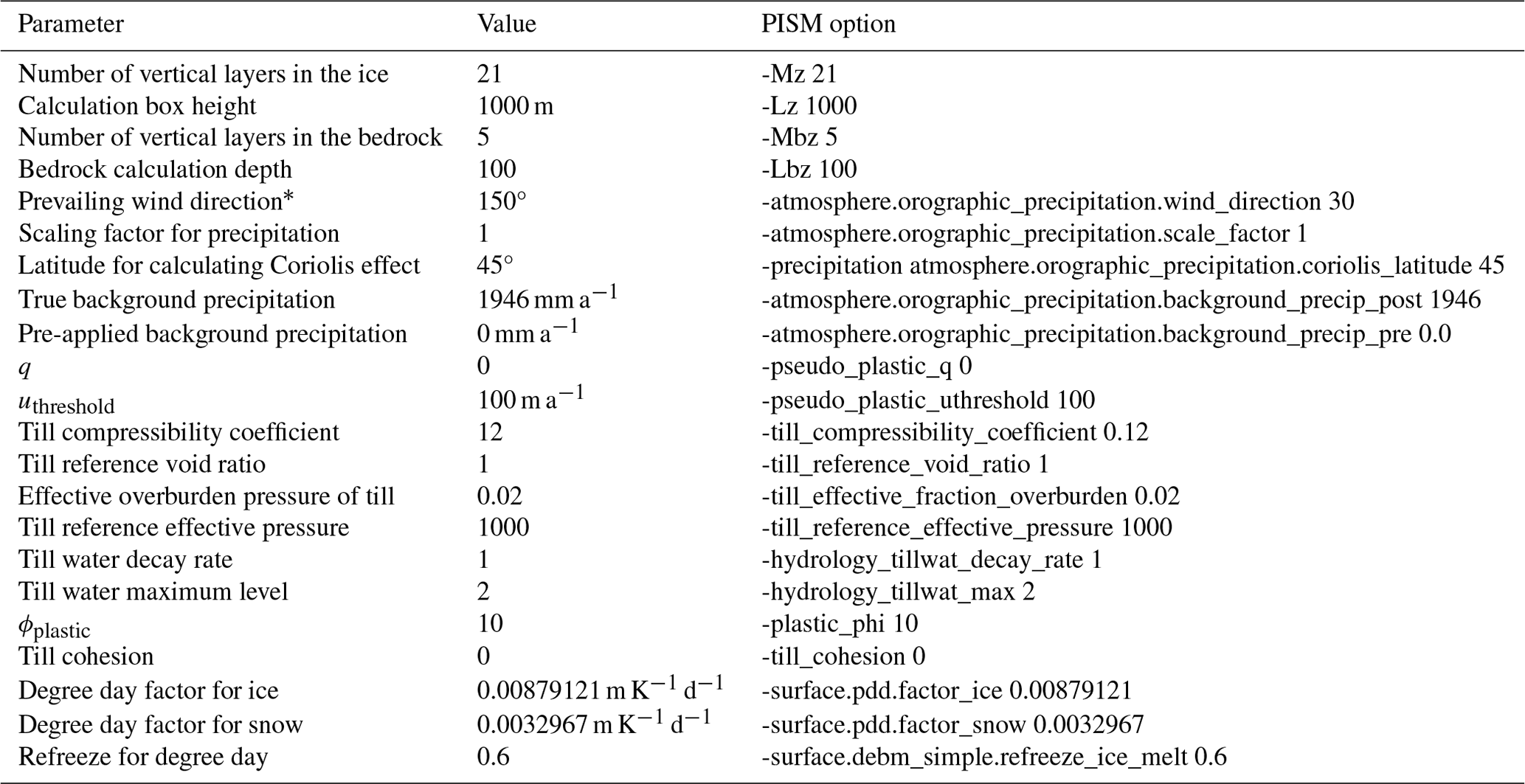
^* Note that the wind direction in PISM seems to ignore the coordinates supplied with DEM and instead assumes some default orientation of the supplied data. We supplied the data oriented differently; therefore, the wind direction had to be remapped.

Table 3 Parameters of custom models and other settings.

3.2 Model domain

The source of the topographical data for the domain is the digital elevation models (DEMs) provided by EU-DEM v1.1 in 50 m resolution from (European Environmental Agency, 2016). To simulate the glacier, a rectangular domain is used that covers the area of about 266 km². For preliminary simulations, the resolutions of either 200 or 150 m had been used, and most of the results presented in the paper have been computed with the resolution of 100 m and in a single case 50 m. Vertically, the ice thickness is limited to 1000 m, and the number of layers is set to 21, resulting in the vertical grid size of the computational box of 50 m. There are also five layers of simulated bedrock, and the total height of the simulated bedrock is 100 m. We experimented also with higher vertical resolutions but observed only a minuscule effect on the simulation results, accompanied with a noticeable increase in execution time. For both the number of ice and bedrock layers, we selected the values based on maximal performance with a satisfactory level of detail, which we determined during preliminary experimentation.

We used grid sequencing, an approach used to decrease the time complexity of steady-state simulations, which is supported by PISM. The simulation is started on a coarse grid for a large portion of simulation time or until a relevant metric, such as the ice volume, converges. Then the grid is refined, and the simulation continues on the finer grid; i.e. the last state of the simulation is interpolated to the finer grid (regridded) and taken as input into the next simulation stage. In the presented study, we used the following setup for grid sequencing, which is based on the empirical values derived from preliminary experiments. Simulations were started on a 400 m grid for 500 years, then continued on a 200 m grid for 1000 years, and finally on a 100 m grid for 1500 years. The final resolution of these simulations was therefore 100 m, as are the resolution of results, while lower resolutions are only used to form rough ice coverage from the initial no-ice conditions.

3.3 Quantitative validation

The main goal of the presented work is to create a computer model that can describe the steady-state ice field under LGM climate conditions. Since the general computer model for ice fields already exists, but the climatic conditions on a microscale are only roughly known, this goal has been translated to a more immediate goal of determining the climatic conditions under which the geomorphological shape of glacier can exist. This goal can be achieved through an optimisation task – a set of input parameters which include the climate forcing has to be continuously tuned (optimised) for the simulations based on them to produce results of increasing quality. The quality of the results can be characterised by how closely the simulated glacier extent aligns with its observed geomorphological form. To provide an objective validation of the simulation result quality, two quantitative metrics have been implemented.

First, a function to determine whether any given coordinate lies inside or outside of the geomorphological glacier area is constructed using both the clear (observed) and unclear glacier boundaries which, used together, bound two separate geographical areas within the domain (see Fig. 1). This function is used to divide the domain into the geomorphological glacier area and the ice-free area. Then, only the clear glacier boundaries are used to generate two artificial border areas, with one bounded by the observed boundary on one side and extending away from the ice field and another bounded by the observed boundary on one side and extending towards the interior of the ice field. These border areas thus represent an area that we are certain was ice-free and an area that we are certain was covered with ice. The simulation should cover the latter with ice but not the former. Therefore, hereafter we name the two border areas forbidden and required, respectively.

Figure 1 General location of the plateau Snežnik (a) and the domain in a resolution of 25 m (b). The geomorphologically reconstructed glacier extent is plotted with dashed (unclear/estimated) and solid lines (clear/observed). The reference weather station and the highest summit of the plateau are marked with a dot and a cross, respectively.

The exact procedure to generate the two border areas is as follows. The clear limits are offset perpendicularly to themselves in both directions (outwards and inwards), creating the boundaries of a singular border area. This is then compared to the geomorphological glacier area, i.e. the area bordered by both clear and unclear geomorphologically reconstructed limits. The intersection of the border area and the geomorphological glacier area then forms the required area, while their difference forms the forbidden area. Since both clear and unclear limits are used in the operation, it is assured that the forbidden area cannot extend into the geomorphological ice field area – even in cases when offsetting the borders of clear limits does so, e.g., in nearby parallel outlet glaciers that exist to the northeast of the presented domain.

The optimisation task for the simulated glacier should minimise the ice coverage of the forbidden area and maximise the ice coverage of the required area. While covered surface areas for border areas could be used in an optimisation procedure directly, we first transform them to relative metrics that are both to be maximised. Therefore, we define two performance metrics, sensitivity Sen and specificity Spe, based on surface areas of the two border areas A_required and A_forbidden:

$$\begin{array}{ll}{\displaystyle }& {\displaystyle }\mathrm{Sen}={\displaystyle \frac{A_{\mathrm{required},\mathrm{covered}}}{A_{\mathrm{required}}}},\\ {\displaystyle }& {\displaystyle }\mathrm{Spe}=\mathrm{1}-{\displaystyle \frac{A_{\mathrm{forbidden},\mathrm{covered}}}{A_{\mathrm{forbidden}}}}.\end{array}$$

When performing the validation of results, sensitivity and specificity are calculated and represent two objectives to be maximised. To illustrate how the metrics are related to the results, we define a simple model of glaciation, where the existence of ice is a function of elevation. Areas above the threshold elevation h are covered with ice, while the others are not, forming an ice field that is highly nonconforming with the geomorphological ice field shape. The relation of the metrics to the thus-defined glaciation is shown in Fig. 2.

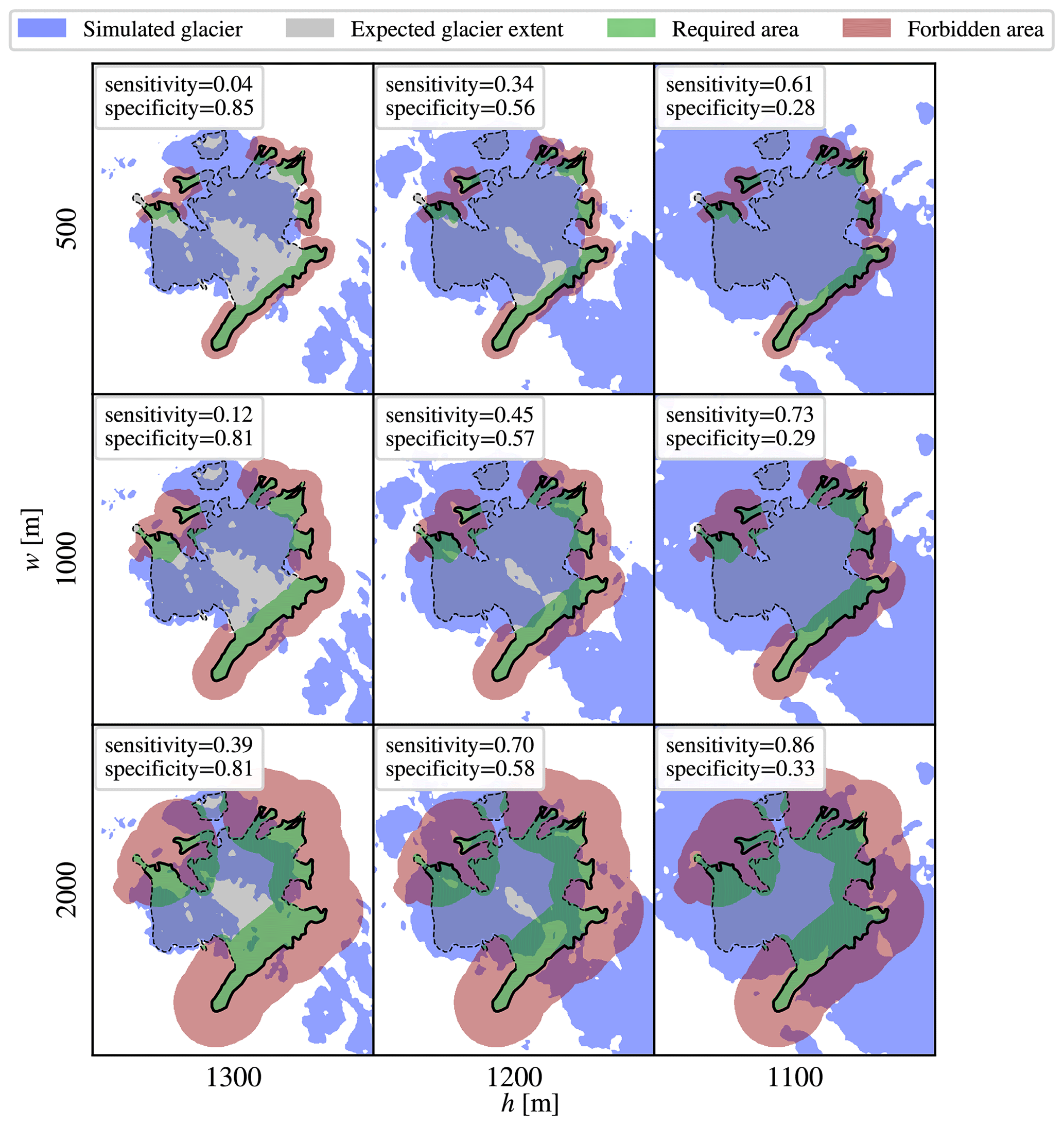
Figure 2 Illustration of the behaviour of quantitative performance metrics, demonstrated on three examples of ice coverage simulated by a simple model, where ice forms above the threshold elevation h but not below. Topology is used in full resolution of 25 m. The metrics are calculated for a varying width of forbidden and required areas w (parameter of the metric) and a varying threshold elevation h (parameter of the simulation).

The amount by which borders are extended inwards and outwards to generate forbidden and required areas is by a parameter that we shall name the width of the respective area hereafter. For simplicity, we shall keep the widths of both areas equal. The presented metrics are a function of width, and thus the metrics can be tuned by adjusting the width, as shown in columns of Fig. 2. As the figure illustrates, a nonconforming ice field shape covers almost indiscriminately both the required and forbidden areas. By increasing the size of a nonconforming shape, both border areas get covered more; therefore, the sensitivity increases but the specificity decreases. The converse is true when the nonconforming shape decreases in size. To truly optimise the shape, one has to find ways to increase both the sensitivity and specificity, which is only possible by transforming the simulated ice field into a more conforming shape.

An optimisation in which there are multiple criteria (or objectives) to be optimised, and these criteria are generally conflicting, is called a multi-objective optimisation (Collette and Siarry, 2004). The problem at hand is a multi-objective problem with two conflicting objectives, and it must be solved as such. We use the “naive” approach (Collette and Siarry, 2004) to solving a multi-objective problem and combine the two objectives into one; we construct the single objective Obj by multiplying the sensitivity and specificity as follows:

$$\begin{array}{}\text{(1)}& \mathrm{Obj}=\mathrm{Sen}\cdot \mathrm{Spe}.\end{array}$$

Then we solve the simpler, single-objective problem by searching for the parameters of simulation that maximise the value of the single objective. Such a combined objective is near zero when one of the factors is near zero; it is higher for balanced than for imbalanced factors (even if their sum is the same), and it increases with the increase in each factor. As such, Obj serves well for optimising the simulated ice field shape to the prescribed form.

So far we have not picked the value for the width – the parameter of both border areas that was shown to greatly influence the resulting sensitivity and specificity. We attempt to optimise the value for width in the following way. To use the presented metrics for quantitative result validation, the width should be large enough to cover the majority of the simulated ice field borders and thus maximise the ability to assign a different numerical value to different results. For example, consider the setting in which the forbidden area extends only 1 km away from the clear boundary. Then, if a simulated glacier extends 2 km over the boundary, it will cause the same drop in the objective function as if it extended only 1 km over the boundary; the results of a clearly different quality will not be discernible through the proposed metrics. Thus, large values of width should be preferred. On the other hand, since the geomorphologically bound ice field is irregularly shaped, increasing the width will result in border areas spreading in such a way that the unclear limits will play an increasingly large part in bounding them. This is not desired; the border area near unclear limits should be minimised to minimise the effect of errors that are likely present in unclear limits.

Three values for the width w are displayed in Fig. 2 for an elevation-based glaciation model, and more were tested in preliminary experiments. The optimal width of border areas takes into account both the preference for large values and the desire to minimise the effect of unclear limits, and according to the scale of the major glacial features on the target area, it seems to be ≈1000 m. From the same figure, trends in sensitivity and specificity as functions of overall ice field extent (characterised by simulation parameter h) can be observed. For all tested values of w, the trends are similar, indicating that the exact value of w might not be important in the context of optimisation. Optimisation works by analysing the difference between the objective values of several simulation results and not on their absolute values. Therefore, optimisation is robust relative to the selection of w and we do not try to fine tune w any further.

3.4 Climate forcing

Climate forcing is implemented through temperature and precipitation models. Both provide location-dependent monthly mean values that are kept constant throughout all the simulated years. Several different models were tested to gain insight into which aspects of climate influence the glacier formation the most and to see how much detail is required for simulations with high fidelity. Within this study, temperature and precipitation models are treated separately, with one having no influence on the other. In this section, two temperature and three precipitation models are presented.

The climate-forcing models are initially tuned to match the modern conditions for which a reference weather station is chosen. This weather station is located in a nearby Mašun, which lies within the area of the Snežnik plateau but outside of the geomorphological area of glaciation (45°37^′41^′′ N, 14°21^′59^′′ E) on 1025 m a.s.l. The station was active between the years 1971 and 1986, and data are available for 97 % of this time range. Monthly mean temperature and precipitation for the station are shown in Fig. 3.

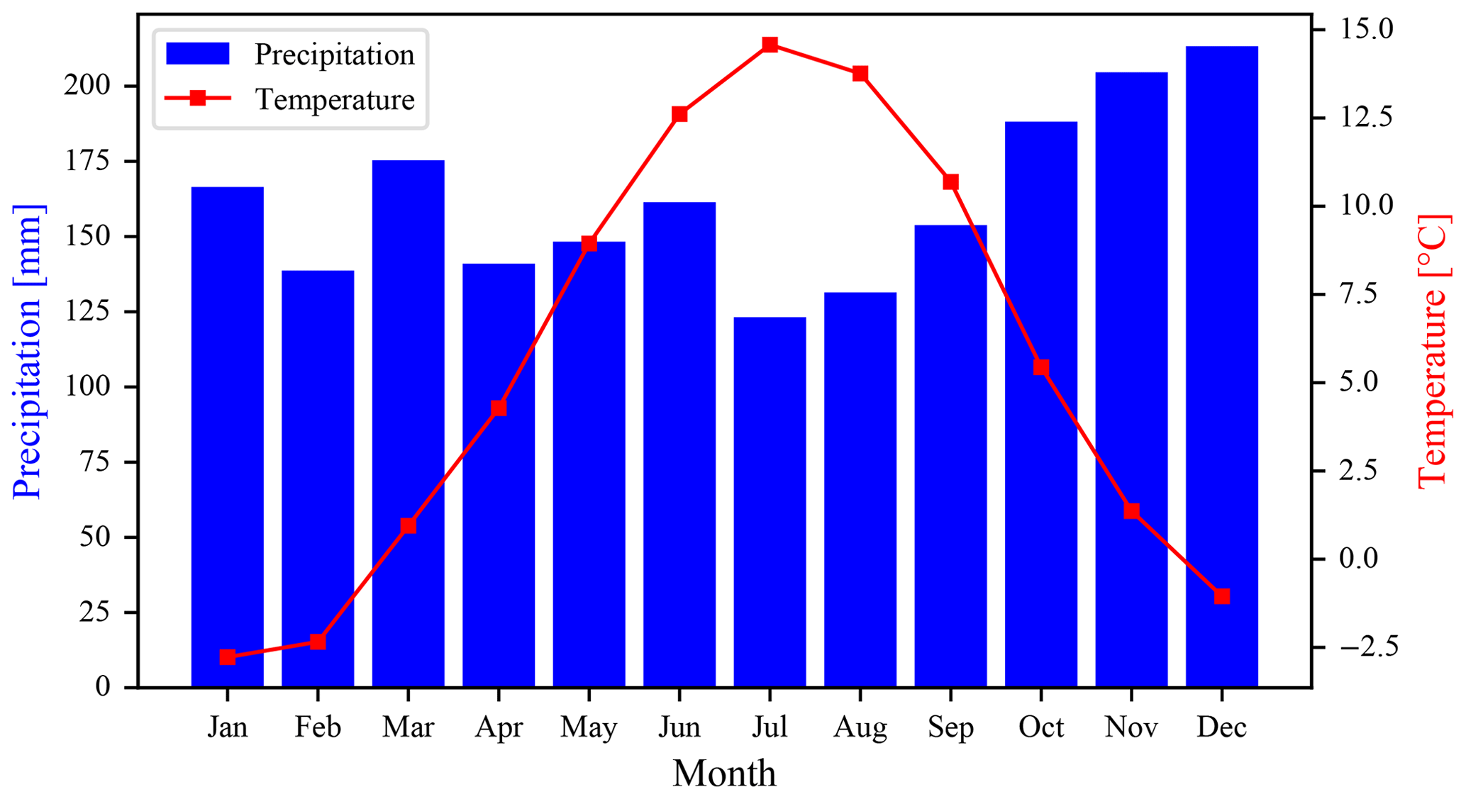
Figure 3 Climate data for Mašun weather station (45°37^′41^′′ N, 14°21^′59^′′ E; 1025 m a.s.l.). The values are averaged for years 1971 to 1986.

In the second step, the models are adjusted to shift the climate towards the LGM. The temperature model output is offset to lower its output by several degrees, while the precipitation model output is multiplied by a factor to cause a relative reduction or amplification, which is then expressed in percentages. The adjustment to temperature and precipitation models is uniform across the domain; i.e. both the temperature offset and precipitation factor are not functions of location. The temperature offset and precipitation factor that form conditions for the optimal ice field are important results of the presented study.

3.4.1 Temperature

The baseline temperature model used in this study – we shall name it the lapse-rate model – comprises a reference point from the reference weather station and the lapse rate for standard atmosphere (Atmosphere, 1975) (6.5 °C km⁻¹) from which temperatures for all grid points can be calculated as follows:

$$T(x,y)={\displaystyle \frac{\left(h\right(x,y)-h_{\mathrm{ref}})}{\mathrm{1000}\cdot \mathrm{6.5}}}+T_{\mathrm{ref}},$$

where h(x,y) is the elevation of each point in DEM, h_ref is the elevation of the reference weather station, and T_ref is the mean temperature recorded at the reference weather station.

The second is an insolation-adjusted lapse-rate model which extends the lapse-rate model with a proxy for the thermal radiation received from the Sun per surface area of the Earth (insolation). The insolation extension is a simplified version of the topographic shading model introduced by Olson and Rupper (2019). It calculates the relative proportion of solar insolation hitting each grid element by projecting the Sun radiance vector to the grid element normal, which is calculated numerically as a pair of symmetric differences through the x and y axis. Therefore, the slopes perpendicular to the incoming radiation from the Sun receive the full relative insolation (value of 1), while slopes parallel to it receive no relative insolation (value of 0). The model of relative insolation S is represented by the following equations (Burrough et al., 2015):

$$\begin{array}{ll}{\displaystyle }& {\displaystyle }\left[\begin{array}{c}\frac{\partial h}{\partial x}\\ \frac{\partial h}{\partial y}\end{array}\right]=\mathrm{\nabla }h(x,y),\forall (x,y)\in \mathrm{DEM},\\ {\displaystyle }& {\displaystyle }\mathit{\alpha }={\displaystyle \frac{\mathit{\pi }}{\mathrm{2}}}-\arctan \left(\sqrt{{{\displaystyle \frac{\partial h}{\partial x}}}^{\mathrm{2}}+{{\displaystyle \frac{\partial h}{\partial y}}}^{\mathrm{2}}}\right),\\ {\displaystyle }& {\displaystyle }\mathit{\beta }={\displaystyle \frac{\mathit{\pi }}{\mathrm{2}}}-\arctan \left({\displaystyle \frac{-\frac{\partial h}{\partial x}}{\frac{\partial h}{\partial y}}}\right),\\ {\displaystyle }& {\displaystyle }S=\sin \left(\mathit{\psi }\right)\cdot \sin \left(\mathit{\alpha }\right)+\cos \left(\mathit{\psi }\right)\cdot \cos \left(\mathit{\alpha }\right)\cdot \sin \left(\mathit{\beta }\right),\end{array}$$

where ψ is the angle of the Sun above the horizon, α is the angle of the slope relative to the horizon, and beta is the aspect angle; i.e. the angle between south and the direction facing the steepest descent from the given coordinates.

Relative insolation S is then multiplied by the insolation effect amplitude A_S to form the equivalent difference in surface air temperature T_S:

$$T_{\mathrm{S}}=A_{S}S.$$

The argument for such a mapping is that a fully insolated area is equivalent to a fully shaded area that is exposed to a higher surface air temperature. This is reflected in the equilibrium line altitude (ELA); i.e. a boundary between the accumulation and ablation areas of the glacier that is very sensitive not only to avalanching, snow drifting, glacier geometry, and debris-cover but also to shading (Nesje, 2014). Geomorphological studies in the nearby Trnovo Forest Plateau by Kodelja et al. (2013) and by Žebre et al. (2013) found out that the difference between the ELA of the sun-facing southern slopes and the shady northern slopes was at least 150 m, while Evans and Cox (2005) set the theoretical boundary of ELA difference at 320 m. The latter limit is used to derive the maximal insolation effect amplitude from the standard atmosphere lapse rate as follows:

$$A_{S,\max }\approx {\displaystyle \frac{\mathrm{320}\mathrm{m}}{\mathrm{1000}\mathrm{m}}}\mathrm{6.5}\mathit{°}\mathrm{C}=\mathrm{2.08}\mathit{°}\mathrm{C}.$$

Note that the calculation of A_S,max should be taken as a rough estimate.

For our further experiments, we used a smaller value of A_S=1 °C, which matches the observed ELA difference better than the upper theoretical boundary. The comparison of temperature fields generated by the models is visualised in Fig. 4. The difference (the insulation part of the model) can be seen to be small and local.

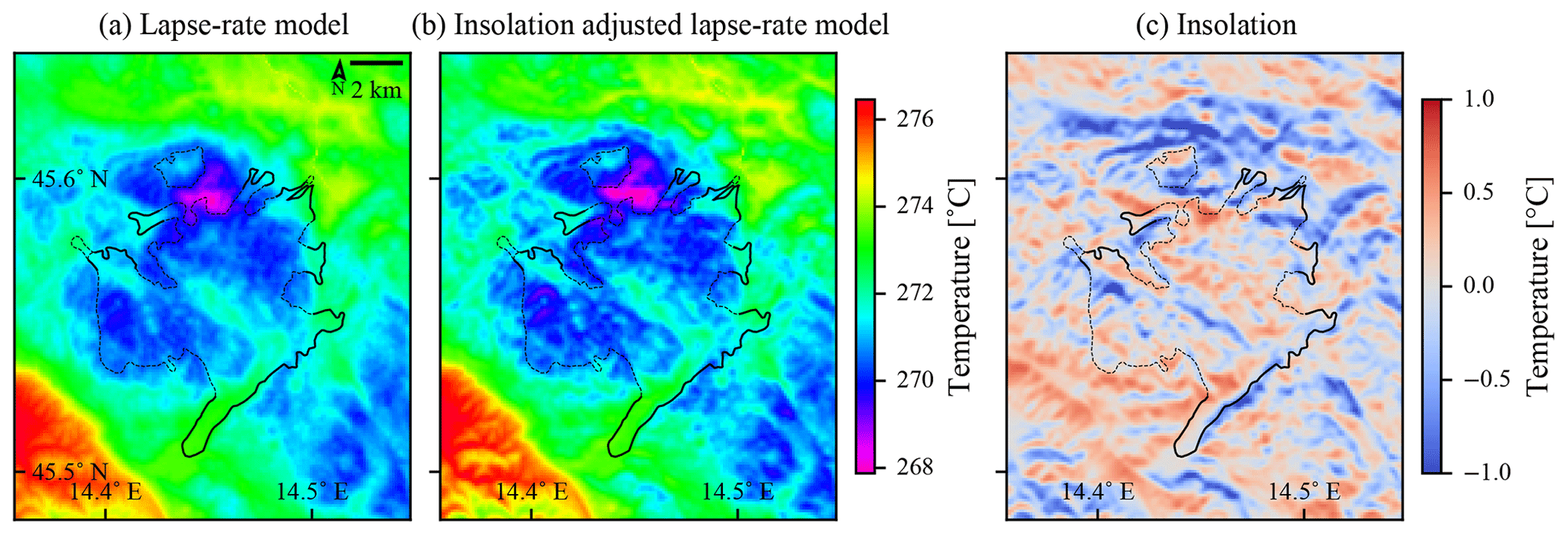
Figure 4 Comparison of the air surface temperature models calculated in the full resolution of 25 m. The generated temperature fields are in panels (a) and (b), while the insolation term of the insolation-adjusted lapse-rate temperature model (which equals the difference between the model outputs) is in panel (c). The geomorphological glacial limits are plotted as black lines.

Finally, temperatures produced by any of the temperature models are offset (decreased) by a constant value, since the present climate is warmer than the simulated past. The preliminary experiments were used to tune the temperature offset to −5.6 °C from the reference average of 1971–1986 to match the simulated glaciation extent with the estimated extent well. This is close to the value of the temperature drop for the larger Alpine area during LGM estimated by Del Gobbo et al. (2023).

3.4.2 Precipitation

Three precipitation models were explored in the presented study. The precipitation fields generated by the three presented models are visualised in Fig. 5 to demonstrate the great difference they produce for the simulation input.

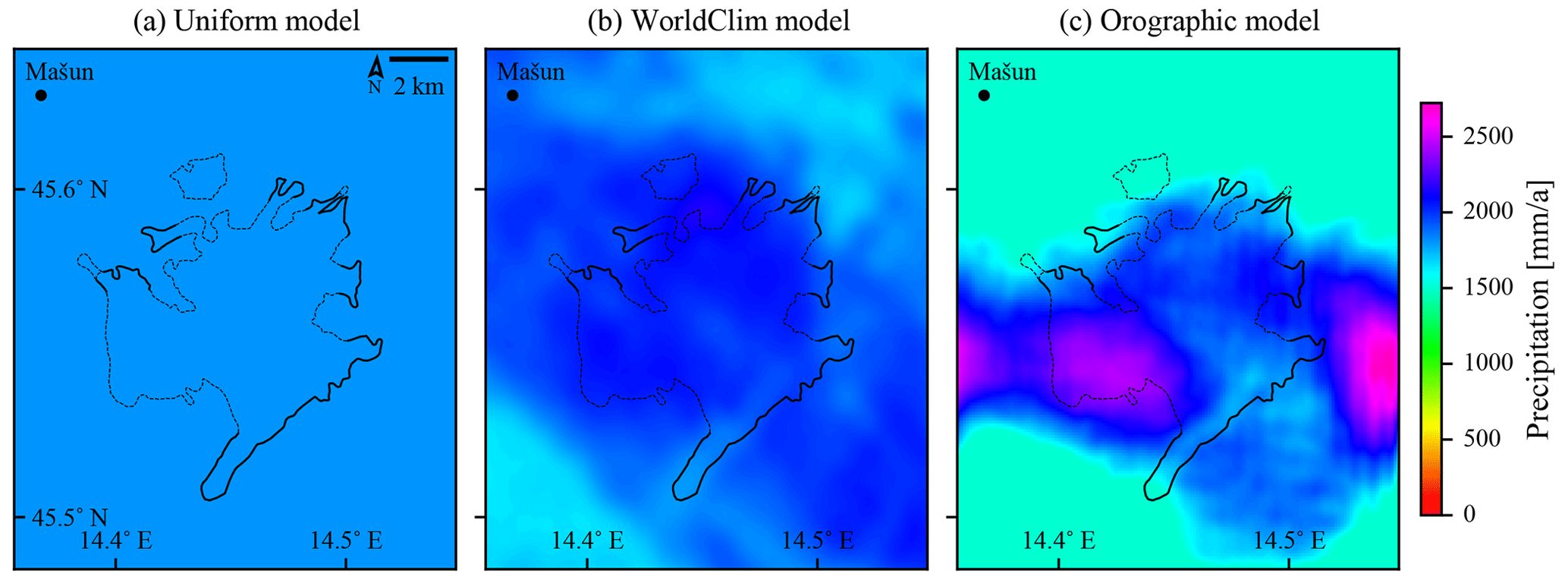
Figure 5 Comparison of the precipitation fields generated by the three described precipitation models. The first two models are pre-calculated as input to PISM and are in the full resolution of 25 m, while the orographic precipitation model is generated by PISM in its working resolution, which was set to 100 m in this case. The field-based estimates of the glacial limits are plotted as black lines.

First is the baseline precipitation model, which assumes uniform precipitations across the domain. The value of the precipitation is taken from the reference weather station and is 1946 mm a⁻¹. Although this is the simplest of models and not appropriate for large areas, it could work in the presented case, since the simulated area is very limited. Note that the used precipitation value also seems low with regard do the larger Snežnik area, with precipitations up to 3000 mm a⁻¹. The reason for this is that the elevation of the station is relatively low, far below the ELA, while the precipitation is expected to increase with elevation. The precipitation pattern generated by this model is shown on the left in Fig. 5.

We shall refer to the second model of precipitation as the WorldClim model, since it originates in an existing global climate model. We use the WorldClim (Fick and Hijmans, 2017) model of global climate as the source, reduce its coverage to the area of the domain, and interpolate (with Lanczos resampling) the mean monthly precipitation component on a 50 m resolution grid (all of the above was done in the software package GDAL). We considered using a local model (Odprti podatki Slovenije, 2023) instead which is based on data gathered by the Slovenian Environment Agency (ARSO) in time interval 1981–2010. We found that the local model did not offer any better resolution, while it failed to cover the whole domain, since a considerable part of the presented domain extends across the national border. The two models also differ notably in their prediction over the selected geographical area, which is clearly observable by the mean annual precipitation over the area enclosed by the geomorphologically determined ice field bounds. For the WorldClim model, the precipitation ranges from 1582 to 1955 mm a⁻¹, with the mean of 1827 mm a⁻¹, which is in contrast to the range from 1950 to 2534 mm a⁻¹, with mean of 2294 mm a⁻¹, for the local model. Thus, the local model prescribes a significantly higher (25 %) precipitation over the critical area for ice field formation. The performed experiments show that the precipitation from the WorldClim model needs to be increased by a small factor for the resulting ice field to be comparable in the ice area to those of other models (the details are available in Sect. 4.4). Therefore, we assume that the WorldClim global climate model underestimates precipitation of the observed geographical area.

The main problem of the climate-model-based precipitation model is that its resolution is far from comparable to the target resolution for the simulations. The best approach to get a better resolution would be to downscale the climate model to the microscale, as there are multiple possible methods for doing so (Maraun et al., 2010); however, even state-of-the-art solutions can only reach resolutions of ≈1 km (Karger et al., 2023), which is still far from the required 100 m. In addition, a downscaling operation would require extensive amounts of data, some of which are only available through proxies and simulations, e.g. palaeoclimate. Therefore, for the purposes of glacial simulation, we currently consider downscaling to the microscale as infeasible. Instead, we perform purely mathematical interpolation of the input precipitation field down to the target grid, which is determined by the target resolution for the simulation at hand. While the interpolated WorldClim model is likely more accurate than the uniform precipitation model, it does not take enough of the local topography details into account and actually leads to a simulation result very similar to the uniform precipitation model (see Fig. 5 for a comparison).

The third precipitation model is based on a physical model, with the measurements only used to estimate some of its parameters. This is the model of orographic precipitation mixed with a uniform precipitation background. Orographic precipitation occurs when moist air is lifted as it moves over a mountain range. As the air rises, it adiabatically cools, and orographic clouds form to serve as the precipitation source. Precipitation then mostly falls upwind of the slope that caused the air lifting. Present-day Snežnik experiences heavy orographic precipitation caused by the south–southeastern moist winds that transport air mass from the nearby Adriatic Sea. Since not all of the precipitation is expected to be of orographic nature, this model mixes it with uniform precipitation across the domain. The main input to the orographic precipitation model is the DEM of the area; thus, the model output can be of the same resolution as the DEM without having to invent the high-resolution details by interpolation. On the other hand, the physics of the model are simplified, and several model parameters have to be invented instead.

To simulate orographic precipitation, the model integrated in PISM is used, which is an implementation of the model by Smith and Barstad (2004) and some of its modifications by Smith et al. (2005). Besides the fixed topology, the main driver of orographic precipitation is wind, which is set up in the model using two parameters – speed and direction. Both parameters are set up as scalar values; the model therefore calculates precipitation for singular weather conditions, which is likely different from the average precipitation. Since the past climate is poorly understood, we do not attempt to set up these two singular parameters from observational and palaeoclimatological data but rather derive them experimentally.

Wind direction is the parameter that influences glacier shape the most; therefore, it represents the first step of the study. First, PISM is set up with the insolation-adjusted lapse-rate temperature model, the uniform precipitation model, and other parameters in a way that results in a glacier of a slightly lesser extent compared to the geomorphological. Then, the simulations are performed with the PISM setup changed to include the orographic precipitation with a varying wind direction by 30°, a constant default wind speed of 10 m s⁻¹, a uniform offset of +3500 mm precipitation (a background precipitation level that can be locally lowered by the orographic precipitation model), and a precipitation factor of 0.5 (which uniformly scales values of individual grid cells of the model output). The listed PISM parameter values can be understood as the background, and orographic precipitation shares being at 50 %, which is our first approximation.

Simulation results are then analysed by comparing their final ice cover, as shown in Fig. 6. The quantitative results of ice coverage comparison are listed in Table 4 and plotted in Fig. 7. Since both sensitivity and specificity should be maximised, the optimal wind angle appears to be 150° (measured clockwise from north), which results in the best trade-off between second-highest sensitivity and very high specificity. Such an angle also seems the best from a visual comparison of the results (which is admittedly a subjective measure) and is furthermore consistent with the direction of the modern precipitation bearing winds.

Figure 6 Influence of the prevailing wind direction on glacier formation. Wind direction is marked in the top-right corners, along with wind roses. The resulting ice coverage pattern is calculated with the presented orographic precipitation model in combination with the adjusted lapse-rate temperature model for non-optimised precipitation and temperature offsets. The resolution of the output is 100 m. The field-based estimates of the glacial limits are plotted as black lines.

Table 4 Ice coverage as a function of wind direction.

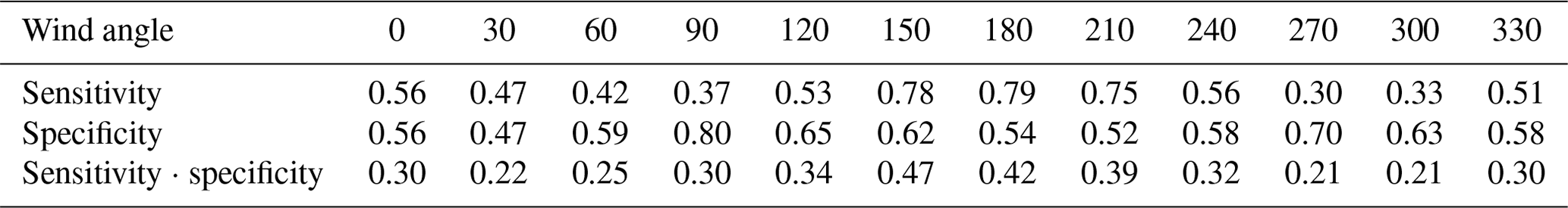
Figure 7 Quantitative metrics for the simulation results of the wind direction parameter sweep. The highest value of sensitivity multiplied by specificity is for a wind angle of 150°.

As the wind direction is selected, other parameters could be optimised further, starting with the most influential ones, namely the wind speed and the ratio between orographic and background precipitation. We feel that a thorough optimisation would be counter-productive though, since a large error is already being made by considering a single wind direction and speed. It should be stressed again that the orographic precipitation model does not consider the wind angle and speed as the mean values but rather as the exact and permanent values. Consider, for example, how the uniformly distributed winds between 120 and 180° instead of the single 150° (the average) wind would generate a very different precipitation field. The same would hold even more so for wind speeds, which are in reality likely to be distributed over a much wider range of values than the wind angle. Therefore, we keep the default wind speed of 10 m s⁻¹ and other parameters of the model (details in Table 2).

Selection of the relative magnitudes of background and orographic precipitation terms was done as follows. Background precipitation was set to equal the measurement at the weather station Mašun (1946 mm a⁻¹), since the latter lies in an area where orographic precipitation does not generate any additional precipitation, and it therefore depends on background precipitation only (see Fig. 5). Then the orographic precipitation was added (unmodified) from the model, resulting in average increase of 323 mm a⁻¹ and a maximum increase of 1526 mm a⁻¹ across the domain. The resulting precipitation is then 2270 mm a⁻¹ on average, with a maximum of 3475 mm a⁻¹, which is in line with the estimated modern precipitation of up to 3000 mm a⁻¹ on average for the Snežnik plateau. Therefore, we treat the precipitation field generated in the way described above as satisfactory and do not optimise it further.

To summarise, the orographic precipitation model assumes a prevailing wind originating from 150°, a wind speed of 10 m s⁻¹, 1946 mm a⁻¹ of background precipitations, and an orographic precipitation model with default parameters as provided by PISM.

In a final note regarding the orographic precipitation model, we should acknowledge that the model was created with a different setting in mind. That is, in the direction from which the wind blows there should preferably be a body of water, or it should at least have uniform elevation and as such also uniform starting moisture content. These two assumptions are a gross oversimplification in our case. The domain could be extended in the direction of the wind to dilute the effect of this error because of the increased distance between the area of interest and the wind origin, but that would increase the error caused by other model assumptions and simplifications. We have performed a preliminary study of how the domain size influences the precipitation pattern over the area of interest. Although the details of the preliminary study are beyond the scope of this study, its results show that changing the domain extent significantly alters the precipitation pattern, but the pattern does not converge when increasing the domain size. Therefore, we use the orographic precipitation model on the presented domain as a demonstration that orographic precipitation is a likely candidate for the observed glacier shape, but we cannot claim so with certainty, nor can we claim that we discovered the exact palaeoclimatic parameters.

From Fig. 5, the orographic precipitation model can be seen to stand out with highest variability across the domain. The patterns of other two models are quite similar within the geomorphological ice field area, which causes the simulation results to be also quite similar, as will be shown later in the paper.

3.4.3 Annual cycles

The above-described climate models are all used to model annual mean temperature and precipitation. The exception may be the WorldClim precipitation model, which can be built to model precipitation at any scale supported by the WorldClim dataset. PISM is adaptable in the way climate data are supplied and can easily work with annual mean data; however, we found in preliminary experiments that simulation results differed greatly when more detailed data, e.g. monthly means, were used instead of the annual data. The likely reason is the monthly variability in the precipitation, which peaks in early winter, as shown in Fig. 3. Consequently, we opted to use monthly means for climate data inputs, and to that end, we apply an annual cycle model on top of previously described models.

The annual cycle model averages monthly values of temperature and precipitation from the reference weather station data and applies them on the temperatures and precipitation modelled by previously described models. The exception is the WorldClim precipitation model, which we constructed from 12 monthly precipitation fields instead of the annual field for the domain, and therefore, it is able to provide monthly values implicitly.

The following procedure is applied to build the annual cycle model. First, the monthly means of temperature and precipitation are taken from the raw weather station data (Fig. 3). Then the monthly mean temperatures are converted into monthly offset from annual mean and monthly precipitations into monthly factor of annual mean. Finally, temperature offsets are applied on the selected temperature model output using PISM's “temperature offsets” and precipitation factors on the selected precipitation model output using PISM's “precipitation scaling”.

4 Results

In this section, we present the results in several forms. First, we confirm that the ice field volume converges, and we provide a time estimate for the convergence to complete. Then we explore how different temperature and precipitation models influence the simulation results, and we comment on which models seem best to use on the presented area. Finally, we present the climate under which we find the optimal conditions for the growth of an ice field in the form that was geomorphologically established.

4.1 Climate setup

The primary objective of this study is to identify the climatic parameters that would allow an ice field atop the Snežnik plateau to align with the extents determined by geomorphological evidence. While this goal will be reached after a large set of experiments have been performed and analysed, a similar goal is set for the first step of experimentation. To even start experimenting with different computational models, since glaciers are not present in the area today, favourable conditions for the formation of glaciers on the domain need to be established first. In other words, the first goal is to set up climatic conditions that would allow for the formation of an ice field similar to the geomorphologically estimated extent.

Using the simplest two models – the lapse-rate temperature model and the uniform precipitation model – a set of simulations has been performed to find suitable starting conditions for further exploration. In Fig. 8, the results of a small grid search with air temperature spacing by 0.5 °C and precipitation spacing of 10 % are shown.

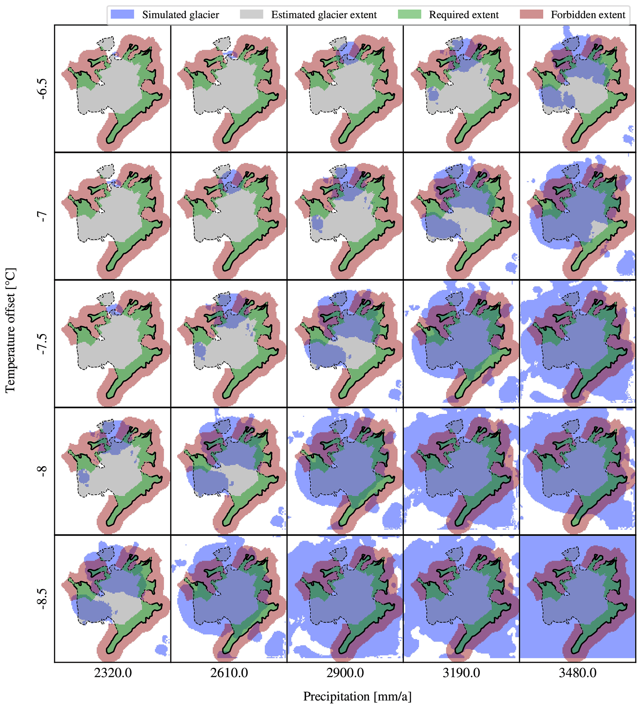
Figure 8 The effect of climate forcings is shown as a matrix of results. The results of the simulations on a uniform precipitation model and a simple temperature model are presented in the resolution that was used for simulations (i.e. 100 m). The field-based estimates of the glacial limits are plotted as black lines. Both parameters can be used to either decrease or increase glacier extent. Furthermore, the results indicate that the parameters are not independent, and the increase in temperature is equivalent to a decrease in precipitation, at least for the range of values shown.

From the figure it is clear that a decrease in temperature of 0.5 °C coupled with a 10 % decrease in precipitation does not significantly alter the extent of the ice field. While these are just human-friendly numbers that were used to set up the parameter scan experiments, we can nevertheless write this observation in a general form:

$$\begin{array}{}\text{(2)}& \begin{array}{rl}I(T,P)& \approx I(T-k_T,k_P\cdot P),\\ & k_T\approx \mathrm{0.5}\mathit{°}C,\\ & k_P\approx \mathrm{0.9},\end{array}\end{array}$$

where I is the ice field that depends on surface air temperature and precipitation fields T and P, respectively, and k_T and K_P are the coefficients representing an approximately 0.5 °C increase in temperature and a 10 % decrease in precipitation. We shall refine the parameters in further experiments, after the confirmation of simulation convergence and the selection of best climate models.

4.2 Convergence

Although various models for temperature and precipitation were used in the preliminary experiments, we only noticed the insignificant influence of the model selection to the convergence of ice volume and ice extent. Therefore, the same settings were used for all the simulations, including the selection of simulated time limits and the number and resolution of simulations within grid sequencing. Figure 9 shows the progression of the ice volume from several experiments that was used to determine the required simulation time and the optimal resolution for further simulations. Note that the shown lengths of the simulation on each individual grid size are different from the values specified in Sect. 3.2, which were selected based on the simulation shown here and other similar experiments, to optimise for the low execution time and satisfactory resolution of the resulting ice cover. From this figure the convergence of solutions towards a steady-state glaciation can be seen, depicting both the time needed for ice accumulation (about 2500 years) and the final volume after it converges (about 2.6×10¹⁰ m³). It can be noted that the resolution of 400 m is not detailed enough, while other tested resolutions all converge to the same volume of ice. A switch from 400 to 200 m could also be done sooner, at 500 to 1000 years, to allow for faster overall convergence. Also, the variation in the ice volume after it has converged can be clearly seen. This means that all further analyses of ice fields that have been performed on a snapshot of the simulation in its final time step will not be perfect, since it is likely that those will focus on slightly different points within the range of the natural variation.

Figure 9 Convergence of the ice field characterised by the ice volume. Presented are four experiments, all using a grid-sequencing approach for faster execution, starting with a resolution of 400 m. The label in the legend specifies the experiment's final resolution. Above the x axis, the grid-sequencing resolutions are specified, and times when resampling potentially occurs are marked with vertical dashed blue lines. Experiments are only resampled to higher resolutions at the resampling times if they have not reached the experiment's final resolution yet. For example, the 200 m experiment starts at 400 m resolution, refines to 200 m resolution at 1500 a, but then remains at that resolution until 4000 a is reached and the simulation is stopped.

4.3 Temperature models

In this subsection, the previously defined temperature models (the lapse-rate model and the insolation-adjusted lapse-rate model; see Sect. 3.4.1) are visually and quantitatively compared, based on simulation results. Experimental simulations are set up to mimic modern precipitation levels, and −6 °C are offset from modern temperatures. Figure 10 shows part of the sensitivity study for the insolation-adjusted temperature model. Only for values of five or greater, which seem unrealistic and are thus not shown in the figure, do the resulting ice field shifts towards the north appear noticeably. Value A_S=0 makes the model behave identically to the lapse-rate model, since the insolation adjustment is multiplied by zero. Then the value A_S=1 represents the case where the solar insolation amplitude is set to mimic the observed ELA difference of 150 m between the insolated and shaded slopes. Finally, the value A_S=3 represents an overvalued effect of insolation.

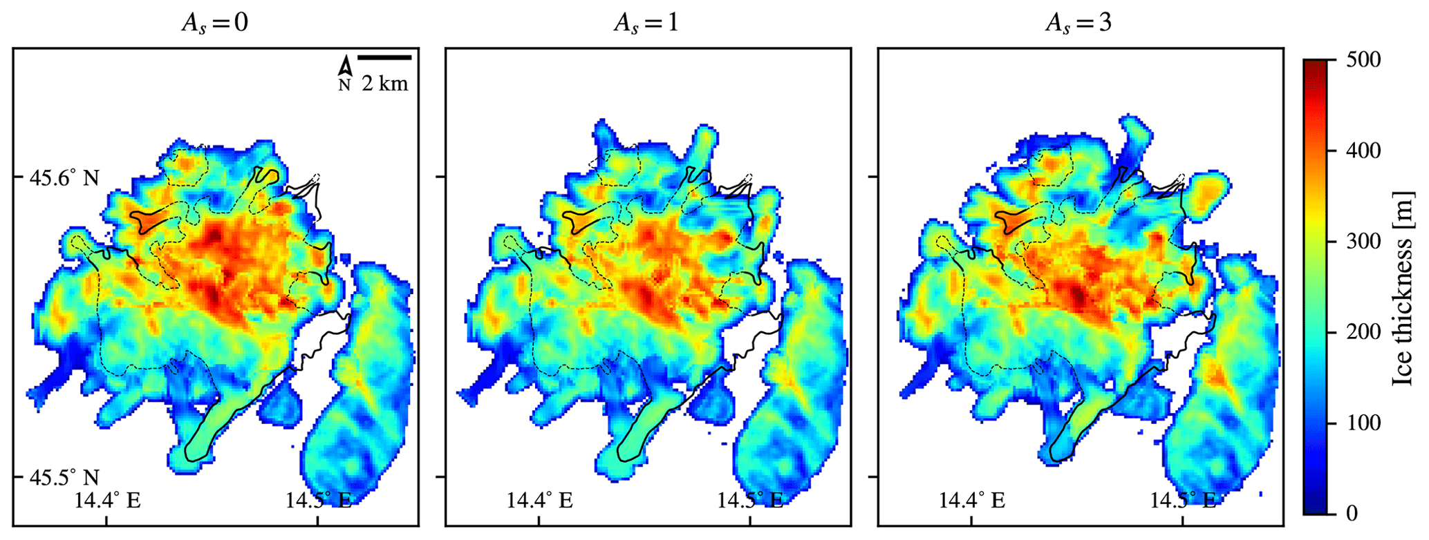
Figure 10 Comparison of the simulation results that use the two presented temperature models and the orographic precipitation model. The geomorphological area of the glacier is outlined in black. The results were obtained using the insolation-adjusted lapse-rate model with three values of A_S, as depicted above the plots. The model with A_S=0 equals a pure lapse-rate model, since the insulation adjustment in that case equals 0 everywhere on the domain. The results are plotted in the resolution used by PISM, which was 100 m in this case, and are contrasted to the field-based estimates of the glacial limits, which are outlined in black lines.

We experimented more with the insolation adjustment than is shown in Fig. 10 but found no significant effect until the A_S is raised very high, e.g. about 5 times its expected value. Similarly, the effect is entirely hidden in the noise if the objective function is observed instead of observing the results visually. Therefore, while our analysis indicates that selecting either of models would suffice for our use case, as they cause only minimal differences in simulation results, we selected the more realistic one; i.e. the insolation-adjusted lapse-rate model with its amplitude parameter A_S set to its most likely value of 1 for further simulations.

4.4 Precipitation models

In this subsection, the differences between the implemented precipitation models (see Sect. 3.4.2) are explored. Selection of the right precipitation model proved to be the most significant one regarding the overall shape of the simulated glacier. Comparison of the simulation results obtained using uniform, WorldClim, and orographic precipitation models is shown in Fig. 11. All three models are set up to mimic modern precipitation levels, and −6 °C are offset from modern temperatures.

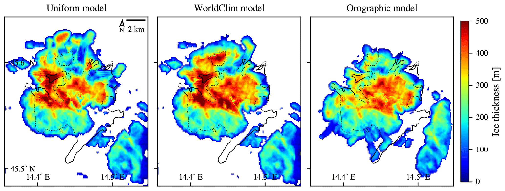
Figure 11 Comparison of the results of simulations that use the three presented precipitation models. Values of the objective for uniform, WorldClim, and orographic models are 0.26, 0.31, and 0.32, respectively. All results are plotted in the resolution of PISM, which was 100 m in this case, and the field-based estimates of the glacial limits are outlined in black lines.

While the quantitative analysis does not show large difference, both constant and WorldClim models cause the ice to grow askew towards the north compared to the geomorphological extent. Under these two precipitation models, the variation in precipitation is very low, and the existence of ice is determined primarily by the temperature model, which in turn is driven by domain elevation. The domain elevation is skewed towards the north compared to the geomorphological ice field position and, thus, so are the simulation results. It should be stressed that the observed north–south imbalance is in addition to and much larger than the one caused by the insolation-adjusted lapse-rate temperature model. Only the orographic precipitation model transfers the distribution of ice southward via precipitation redistribution.

Unlike the visual inspection, the value of the objective is only slightly higher for the orographic model (0.32) than for the other two models (0.26 and 0.31). The larger ice field located to the southeast is partially responsible, which covers the largest part of forbidden area in the simulation with orographic precipitation model. The ice field to the southeast is part of an area otherwise known as Gorski Kotar (Žebre and Stepišnik, 2016), and is expected to glaciate in simulations, but was not a part of the performed study. The isolation of the two ice fields is clear from the performed geomorphology studies. Its proximity, however, makes the analysis of Snežnik in isolation more demanding. This case therefore highlights a disadvantage in the presented quantitative measure – the unmarked proximal ice fields may have a significant impact on the accuracy of the qualitative measure.

Nevertheless, orographic model is best both visually and quantitatively and is selected as the base precipitation model to be used for further simulations of this geographical area.

4.5 Climate conditions for Snežnik

In this subsection, we present the results that to some extent address the goal of the study – improving our understanding of the past climate–glacier dynamics at the Alps–Dinarides junction. There are two main results. First, we establish that the problem is underdetermined, and we can provide optimal climate conditions for the formulation of an ice field on the Snežnik plateau only as a linear relation. Second, we find one set of climate conditions that respect both the linear relation from the first result and the state-of-the-art global climate estimates. We present the modelled ice field under such climate conditions on the domain with a resolution of 50 m.

First, an experiment has been prepared to obtain one set of climate conditions under which the simulated extent matches the geomorphological extent the best. Since the temperature and precipitation have been found to be related, a fine-grained grid search has been performed on air temperature only, with the precipitation fixed to modern values. The main results are summarised in Fig. 12 in the form of the objective values for all performed simulations and in Fig. 13 in form of ice extents of the nine best-performing simulations. Visually, the shown extents are difficult to order by quality. Some of the ice field features, e.g. termini, are better covered at higher temperature, while others are covered at a lower temperature. Looking at the value of the objective, small differences can be made out, and the objective value peaks at the −5.6 °C surface air temperature offset, although the differences compared to other offsets are small. The result would be perfectly acceptable if the air temperature is either increased or decreased up to 0.2 °C with only a different trade-off between sensitivity and specificity.

Figure 12 Value of the objective for the fine-grained sweep over the temperature with a fixed precipitation value. The highest value of the objective (sensitivity multiplied by specificity) is at −5.6 °C.

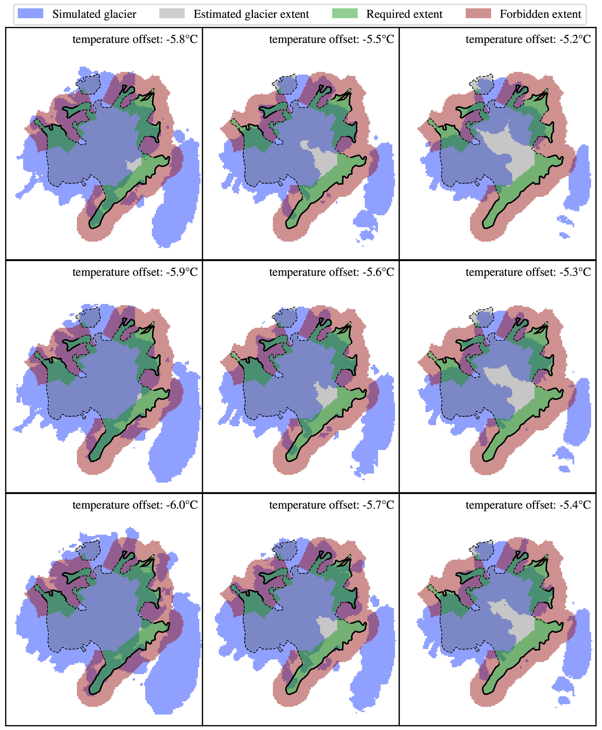
Figure 13 A fine-grained sweep over a single parameter – near-surface air temperature. The objective measure for the ice cover is given in Fig. 12. All results are plotted in the resolution of PISM, which was 100 m in this case, and the field-based estimates of the glacial limits are outlined in black lines.

Using the obtained set of best climate conditions, the simulated ice field extent is examined in more detail. The resolution of 50 m is computationally too expensive to be used for the exploration of the climatic conditions while providing results that are only marginally better then those obtained by 100 m resolution. It has been selected for the final simulation along with the climate conditions defined above, since it provides some additional detail, especially in the ice flux. Ice flux in the final state of the simulation is shown in Fig. 14. The simulation shows that the ice flow patterns on Snežnik are largely controlled by the subglacial topography. The glaciated area is composed of two plateaux above 1300 m that behaved as accumulation areas from where the ice was flowing almost radially downstream. The ice from the northern and southern plateau joined in a large karst depression in between them; from there, it was drained by an outlet glacier flowing towards south/southeast. This is in agreement with the geomorphological evidence, despite some discrepancies between the simulated and geomorphological ice extent.

Figure 14 Streamlined plot of the ice flux (arrows) overlaying the ice thickness and the geomorphological ice field outline (thick lines for the clear outline and dashed lines for the unclear outline). The experiment was performed on a domain with a 50 m resolution.

Last, we look into the relationship between temperature and precipitation. As seen in Fig. 8 and described in Eq. (2), any increase in precipitation can be countered by a decrease in temperature to keep the conditions for simulated glacier formation about the same. Using the best temperature and precipitation models, we have performed additional experiments to improve the approximations for coefficients of Eq. (2) and found that the values of k_T=0.45 and k_P=0.9 are nearly optimal. Based on the Eq. (2) and the experimentally discovered optimal coefficient values, the final equation describing the optimal conditions can be written with x being the free parameter:

$$\begin{array}{}\text{(3)}& \begin{array}{rl}& T=-\mathrm{5.6}\mathrm{°}\mathrm{C}-x\cdot \mathrm{0.45}\mathrm{°}\mathrm{C},\\ & P=\mathrm{1946}\mathrm{mm}{\mathrm{a}}^{-\mathrm{1}}\cdot {\mathrm{0.9}}^x,\\ & x\in \mathbb{R}\mathrm{and}x\mathrm{is}\mathrm{small}.\end{array}\end{array}$$

To confirm that climate conditions that conform to Eq. (3) result in similar ice fields, we have designed an additional experiment. For a limited set of values x, the ice field is simulated, and the results are compared to the results simulated at x=0 according to the defined objective. The results of the experiment are presented in Figs. 15 and 16. Besides confirming the equation, the described experiment also gives a range of valid values for x, where Eq. (3) holds.

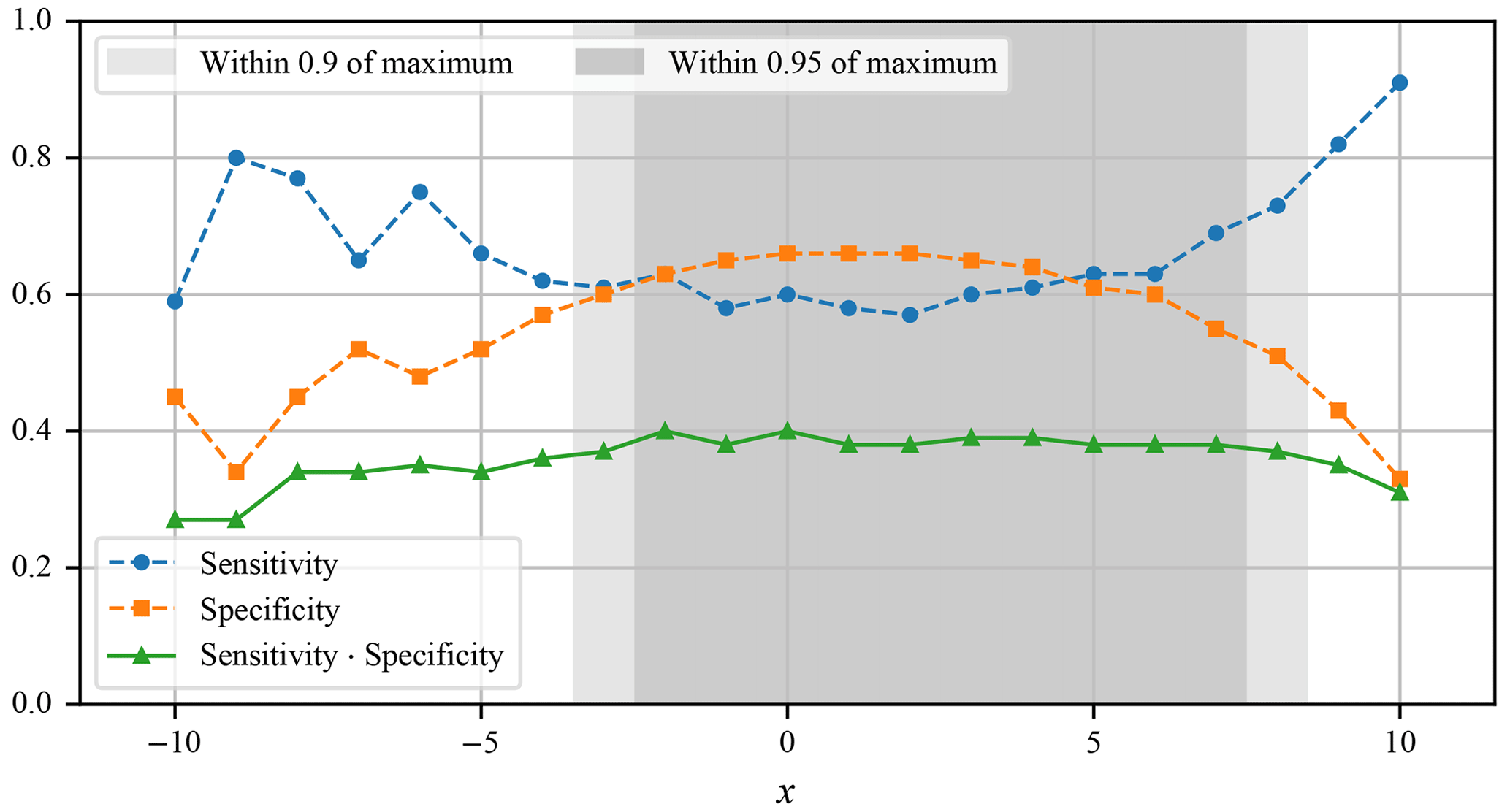
Figure 15 Relation between the free parameter of Eq. (3) and the objective value. The shaded areas represent solutions where the value of objective function is within 90 % and 95 % of the maximum obtained value.

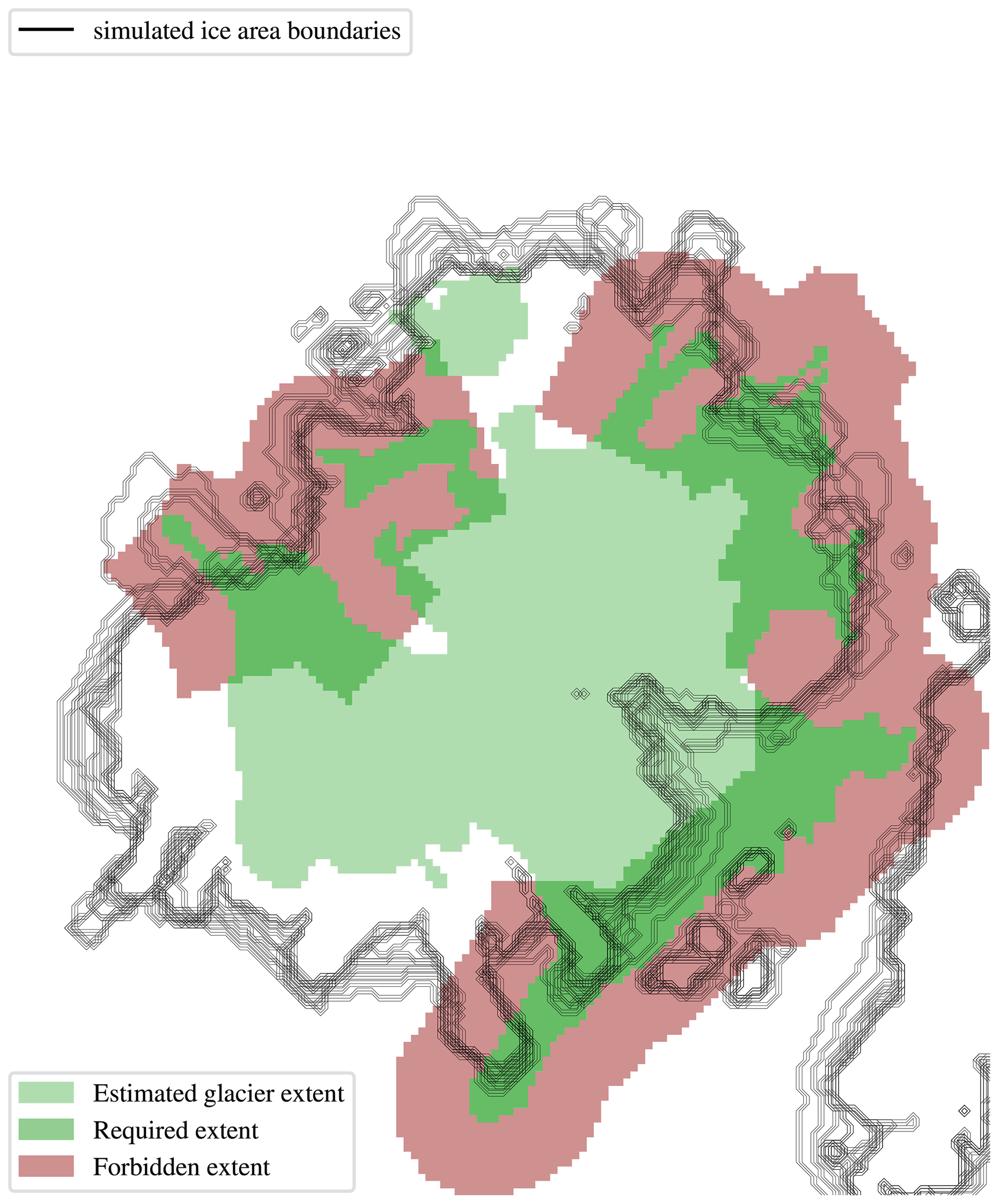
Figure 16 Outlines of simulated ice fields for the values of $x\in [-\mathrm{3},+\mathrm{8}]$, for which the value of objective function is within 90 % of the maximum obtained value plotted with black lines. All simulations for this figure were calculated with the PISM resolution set to 100 m.

The range of x seems to be based on the interval $[-\mathrm{3},+\mathrm{8}]$ from the selected reference point. Therefore, one can take a valid value of x=3.11, which is within this interval, to get the temperature offset of −7 °C and a precipitation factor of 0.66 relative to modern conditions. Adjusting the temperature offset by the previously mentioned 0.4 °C of difference between our modern reference interval and the pre-industrial era, the temperature offset exactly matches the results of Del Gobbo et al. (2023), who reconstructed the LGM temperature to be offset by −6.6 °C relative to pre-industrial era. The precipitation of 0.66 relative to the modern reference interval is also close to the reconstructions by Del Gobbo et al. (2023), where the precipitation for the general area is estimated to lie between −10 % and −30 % relative to the pre-industrial.

5 Discussion and conclusions

Several results of the presented study are summarised and discussed below. First, a qualitative metric of the simulation quality was developed, which can take clear and unclear geomorphologically deduced ice boundaries into account. Second, the relation between precipitation and temperature was quantified. Third, several simulations resulting in an appropriately sized ice field were successfully performed using climatic forcing compatible with LGM conditions. Last, the factor with the largest effect on the simulation results was found to be the precipitation pattern. Global precipitation models, such as the one provided by WorldClim, were found to be insufficient for simulation of accurately shaped ice fields. On the other hand, even the simplest temperature models, such as one based entirely on elevation and lapse rate, were sufficient for our use case.

This research has successfully established a quantitative framework for the assessment of palaeoglacial simulations that integrates both definitive and provisional geomorphologically deduced ice boundaries to improve the accuracy of model results. The developed qualitative metrics help determine the agreement between the model-derived ice extents and those derived from geomorphological field data.

The framework alleviated the difficult task of sorting the simulation results by quality but did not eliminate visual checks entirely. The reason lies in its shortcomings, which we list here. First, its parameters are required to be set up, which in turn requires experimenting. In the presented case, the experimenting was light but could have proven more difficult for a more demanding ice field shape. Second, the framework is missing a methodology for ignoring neighbouring glaciated areas. We expect that neighbouring glaciations can often be a problem since the simulator requires the domain to be rectangular and to be somewhat larger than the area of interest. Thus, it is likely for most studies to find that their domains contain some glaciers that are outside of the focus and require special treatment in the analysis. Finally, the proposed framework is very specific in its demands for at most two types of limits – clear and unclear. There is currently no room for quantifying the clarity nor for including more limit types. While this framework would work if only clear limits were given, such cases could also make use of simpler analysis methods.

The framework, along with visual analysis, aided in deciding on the best climate models and in optimising ice field reconstructions towards conformity with the geomorphological bounds. The reconstructions resulted in the demonstration of the relation between air temperature and precipitation when it comes to the size of glaciers. These two factors affect each other in a way that creates a balance within the simulations causing different combinations of temperature and precipitation to result in similar glacier extent. This interplay precludes the determination of exact climatic conditions based on glacier morphology alone and suggests a broader framework of possible past climates that are consistent with the observed glacier extent. This study formulates the interplay as a pair of equations with a single independent variable. Furthermore, it quantifies the parameters of equations and bounds them to a range of values beyond which the interplay gradually loses its effect.

The presented relation between temperature and precipitation presents a degree of freedom that can only be resolved by additional external data. The latest reconstructions of LGM climate (Del Gobbo et al., 2023) are a great source for external data, and the proposed relation between temperature and precipitation matches this particular data point well. Simulations carried out under the climatic conditions of the LGM suggest an ice field that is broadly consistent with empirical geomorphological reconstructions. The consistency is limited to the ice field size, however, as the simulations fail to reproduce all the bounds of the geomorphologically reconstructed ice field. Although the established framework aided in the optimisation of the unbound parameters in climate models, some systematic biases remain in the simulations. These could be resolved in the future by more detailed climate models. The precipitation model was a key component in the presented study and remains a candidate for further improvements.

Another area where improvements should be sought is in optimising the values of various unmentioned model parameters. Within the preliminary analysis of climate models, we explored the sensitivity of the simulated ice field area and volume with varying modelling parameters such as those related to the domain grid, ice rheology, stress balance, basal sliding, and till properties. Our findings are consistent with those from studies published by Žebre et al. (2021) and Candaş et al. (2020). Specifically, the simulated glaciation extent and volume are as sensitive to choices related to parameterisation of other models, as they are to climate models. This sensitivity suggests that small variations in parameters can lead to significant differences in the results. Given this, along with the lack of local measurements to aid in parameter adjustments, the presented results should be interpreted with due caution. For future work, a methodology to set up or optimise all the major model parameters should be developed.

Another finding of this research is the disproportionate influence of precipitation patterns on the simulation results. It was found that the spatial distribution of precipitation, especially when influenced by orographic factors, is crucial for the accurate representation of glacier extent. It has been shown that global precipitation models such as WorldClim do not have the necessary resolution nor the orographic sensitivity to accurately simulate the shape of ice fields. This inadequacy requires the integration of high-resolution topographic data and locally refined precipitation data to capture the complex interactions between topography and climate. We must bear in mind that the orographic precipitation model is based on assumptions about wind patterns that may not accurately reflect the complex interactions between topography and climate, especially given the lack of palaeoclimatic data on wind direction. As a phenomenon that is underrepresented in models but has a demonstrated high influence on results, wind should represent an area of additional research in the future.

Conversely, the adequacy of elementary temperature models relying solely on lapse rates and elevation data reveals the relative insensitivity of the studied ice field extent to the temperature data. This observation points to a potential area of computational optimisation in modelling efforts where high-resolution temperature data are not readily available.

Although advanced, the presented climate models used may still be an oversimplification of actual past conditions. The temperature model could be improved using mountain shading, in addition to insolation adjustment, and a orographic precipitation model could be extended to include a set of most typical wind conditions. There is also the option of extending the till and hydrology models based on additional field observations to better simulate the karst conditions of the researched geographical area. On the other hand, the existing simulations can be used to find additional evidence of glaciation in the field to better constrain the next iteration of the simulation. While a larger area of Snežnik has already been mapped, and every standard-sized landform has been mapped, there is still much that is unknown when it comes to the sediment filling of karst depressions. The existing best-fit simulations could potentially help locate points of interest for further research, e.g., to plan drilling into the sediments trapped in karst depressions close to the simulated ice boundary.