New estimation of critical insolation–CO₂ relationship for triggering glacial inception

It has been previously proposed that glacial inception represents a bifurcation transition between interglacial and glacial states and is governed by the nonlinear dynamics of the climate–cryosphere system. To trigger glacial inception, the orbital forcing (defined as the maximum of summer insolation at 65° N and determined by Earth’s orbital parameters) must be lower than a critical level, which depends on the atmospheric CO₂ concentration. While paleoclimatic data do not provide a strong constraint on the dependence between CO₂ and critical insolation, its accurate estimation is of fundamental importance for predicting future glaciations and the effect that anthropogenic CO₂ emissions might have on them. In this study, we use the novel Earth system model of intermediate complexity CLIMBER-X with interactive ice sheets to produce a new estimation of the critical insolation–CO₂ relationship for triggering glacial inception. We perform a series of experiments in which different combinations of orbital forcing and atmospheric CO₂ concentration are maintained constant in time. We analyze for which combinations of orbital forcing and CO₂ glacial inception occurs and trace the critical relationship between them, separating conditions under which glacial inception is possible from those where glacial inception is not materialized. We also provide a theoretical foundation for the proposed critical insolation–CO₂ relation. We find that the use of the maximum summer insolation at 65° N as a single metric for orbital forcing is adequate for tracing the glacial inception bifurcation. Moreover, we find that the temporal and spatial patterns of ice sheet growth during glacial inception are not always the same but depend on the critical insolation and CO₂ level. The experiments evidence the fact that during glacial inception, ice sheets grow mostly in North America, and only under low CO₂ conditions are ice sheets also formed over Scandinavia. The latter is associated with a weak Atlantic Meridional Overturning Circulation (AMOC) for low CO₂. We find that the strength of AMOC also affects the rate of ice sheet growth during glacial inception.

1 Introduction

Glacial cycles are the dominant mode of climatic variability over the last 2.7 million years. The timing of glaciations and deglaciations is primarily controlled by changes in Earth’s orbital parameters through the modulation of the amount of solar radiation received in high latitudes of the Northern Hemisphere (NH) during boreal summer (Milankovitch, 1941; Ganopolski, 2024).

Using an Earth system model of intermediate complexity (EMIC), Calov et al. (2005) proposed that glacial inception represents a bifurcation transition from interglacial to glacial states of the Earth system. When summer insolation at high latitudes of the NH falls below a certain threshold, the interglacial state becomes unstable and ice sheet growth begins. The process is amplified through nonlinear feedbacks, among which the snow and ice albedo and the elevation feedbacks are the dominant ones. Eventually, large ice sheets develop over the North American and Eurasian continents.

The threshold value for boreal summer insolation to trigger a glacial inception depends on the atmospheric concentration of greenhouse gases, among which CO₂ is, by far, the most important (Köhler et al., 2010). While paleoclimatic data do not constrain this dependence, its accurate estimation is of fundamental importance for predicting future glaciations and the effect that anthropogenic CO₂ emissions might have on them (Archer and Ganopolski, 2005; Talento and Ganopolski, 2021).

The first attempt at tracing the relationship between insolation and CO₂ for triggering glacial inception was performed in Archer and Ganopolski (2005) using the EMIC CLIMBER-2 (Petoukhov et al., 2000; Ganopolski et al., 2001). This first estimation was, however, rather crude as it was based only on a small set of relatively short experiments that did not allow for the detection of the bifurcation with sufficient accuracy. Ganopolski et al. (2016) updated the results also using CLIMBER-2 with a new methodology that allowed for increased accuracy. The authors proposed a functional relationship between summer maximum insolation at 65° N (smx65) and CO₂ for triggering glacial inception. The relationship describes the critical smx65 for the onset of glaciation as linearly dependent on the logarithm of CO₂: smx65${}_{\mathrm{cr}}=\mathit{\alpha }\ln ({\mathrm{CO}}_{\mathrm{2}}/{\mathrm{CO}}_{{\mathrm{2}}_{\mathrm{0}}})+\mathit{\beta }$, where CO₂ is the atmospheric CO₂ concentration, ${\mathrm{CO}}_{{\mathrm{2}}_{\mathrm{0}}}$ is a reference atmospheric CO₂ value (the pre-industrial value), and α and β are empirical constants.

The shape of the dependency is in agreement with the facts that (i) the radiative forcing of CO₂ follows a logarithmic structure and (ii) that in CLIMBER-2 the temperature response to radiative forcing of CO₂ and orbital forcing is linear within the considered range.

The purpose of this work is to build upon the findings of Ganopolski et al. (2016) and generate a new estimation of the relationship between insolation and atmospheric CO₂ critical for triggering glacial inception using the recently developed and more advanced CLIMBER-X model (Willeit et al., 2022, 2023, 2024). While CLIMBER-X is also an EMIC that shares with CLIMBER-2 the principles of computational efficiency and usage of a statistical–dynamical atmospheric model, it represents a significant development compared to the CLIMBER-2 model used in previous studies (Ganopolski and Brovkin, 2017; Willeit et al., 2019). In particular, CLIMBER-X has (i) a much higher horizontal resolution in the atmosphere and land models (5° × 5° versus ∼ 50° × 10° in a longitude–latitude grid), (ii) a 3D ocean model, (iii) more internally consistent components, and (iv) better treatment of individual processes (e.g., surface energy balance, precipitation, radiative transfer, sea ice dynamics, photosynthesis, vegetation dynamics). Furthermore, we investigate the temporal and spatial patterns of ice sheet growth during glacial inception and the effects of changes in the Atlantic Meridional Overturning Circulation (AMOC) strength on the rate of ice sheets growth. We also analyze the suitability of using the smx65 as a single metric for orbital forcing. A theoretical derivation of the critical insolation–CO₂ relationship for triggering glacial inception is provided in Appendix A.

2 Model and experimental setup

2.1 Model description

We employ the new CLIMBER-X EMIC (Willeit et al., 2022, 2023, 2024). The model was specifically designed to simulate the Earth system evolution on timescales from decades to hundreds of thousands of years. The climate component of CLIMBER-X consists of the 2.5-dimensional Semi-Empirical dynamical-Statistical Atmosphere Model (SESAM), the 3-dimensional frictional–geostrophic ocean model GOLDSTEIN, the dynamic–thermodynamic SImple Sea Ice Model (SISIM) and the land surface–vegetation model PALADYN. All the models from the climate core are discretized on a longitude–latitude grid with 5° × 5° horizontal resolution and use a daily time step. The ocean model has 23 unequally spaced vertical layers, with a 10 m top layer and layer thickness increasing with depth and reaching 500 m at the ocean bottom. CLIMBER-X incorporates the 3-dimensional thermomechanical ice sheet model SICOPOLIS (Greve et al., 2017) via the high-resolution physically based surface energy and mass balance interface SEMIX (Willeit et al., 2024) and a basal ice shelf melt module. In this study, SICOPOLIS is applied only to the NH with a 32 km horizontal resolution. The viscoelastic solid Earth model VILMA (Klemann et al., 2008; Martinec et al., 2018) is used to simulate the bedrock response to changes in loading by solving the sea level equation. A detailed description of the coupling between climate and ice sheet components is provided in Willeit et al. (2024). CLIMBER-X does not simulate internal decadal-scale variability by its design, but it can simulate the forced response at this timescale, such as response to volcanic eruptions and CO₂ changes (Willeit et al., 2022). The equilibrium climate sensitivity of CLIMBER-X is ∼ 3 °C, close to the best-guess estimate from the IPCC (IPCC 2021, 2021).

Even though CLIMBER-X has a relatively coarse spatial resolution and a simplified treatment of some processes, the number of physical processes included in the model and its performance for the present-day climate are comparable with state-of-the-art (CMIP6-type) climate models (Willeit et al., 2022, 2023). CLIMBER-X is reasonably successful in reproducing the present-day climatology of variables relevant for the formation of ice sheets. However, near-surface summer temperatures (a key variable for determining ablation of ice sheets) are up to 5 °C too warm over the eastern portion of North America when compared to observations (Willeit et al., 2024). Preliminary experiments show that such biases preclude the realistic development of North American ice sheets. Therefore, similarly to Ganopolski et al. (2010), we implemented a 2 m temperature bias correction in the surface mass balance calculation (see Willeit et al., 2024). In addition, a uniform offset of −0.5 °C is applied globally in the surface mass balance scheme. As discussed in Willeit et al. (2024), the precipitation biases in CLIMBER-X are less problematic for the simulation of the surface mass balance of NH ice sheets.

2.1.1 Experimental setup

We perform a series of equilibrium experiments in which different orbital parameters (obliquity, eccentricity and precession) and the atmospheric CO₂ concentration are maintained constant for the whole duration of the simulation. All NH ice sheets are fully interactive and influence climate through albedo, elevation, sea level (which affects the land–sea mask) and freshwater flux into the ocean (Willeit et al., 2024). Since the ocean model in CLIMBER-X is based on the rigid-lid approximation we always enforce the net annual global surface freshwater flux being zero. In the case of interactive ice sheets, we still enforce the global annual surface freshwater flux being zero but then adjust the ocean volume each year to match the change in global ice volume (Willeit et al., 2022). The Antarctic ice sheet is not interactive but fixed at its present-day state. The experiments are performed using an acceleration technique with asynchronous coupling between the climate and ice sheet model components. An acceleration factor of 10 is used; i.e., the climate model component is updated every 10 years of the ice sheet model. If we were to calculate global ocean volume change by integrating surface freshwater fluxes, then a 10-fold acceleration would require us to aggregate these fluxes over 10 years, but since in our model the ocean volume change is not driven by surface freshwater fluxes this is not necessary and the freshwater fluxes are computed as in the non-accelerated case. Willeit et al. (2024) demonstrated that acceleration factors up to ∼ 10 are acceptable and provide realistic results of the last glacial inception. Each model simulation is run for 100 000 years of the ice sheet model (corresponding to 10 000 years of the climate model) starting from pre-industrial equilibrium conditions with the observed present-day Greenland ice sheet with a uniform ice temperature of −10 °C.

We select 19 combinations of orbital parameters corresponding to the 19 local minima of the smx65 time series of the last 400 kyr, corresponding to values in the range between 430 and 496 W m⁻² (Fig. 1). Therefore, selected combinations of orbital parameters have similar precession but very different eccentricity and obliquity values. For each of these 19 sets of orbital parameters, we produce a series of equilibrium experiments designed to detect the critical insolation–CO₂ relationship for triggering inception. The procedure is, for each set of orbital parameters, as follows.

1. We start from a simulation using a (fairly high) atmospheric CO₂ concentration of 500 ppm, for which glacial inception is not expected to occur under any orbital configuration.

2. If the NH ice volume (v) is <X m s.l.e. (meters in sea level equivalent) during the whole simulation, we reduce CO₂ by 5 ppm and repeat the simulation.

If, on the contrary, v is ≥X $\mathrm{m}\mathrm{s}.\mathrm{l}.\mathrm{e}.$ at any moment in the simulation, we stop the iteration and define the insolation–CO₂ combination used in this case as critical for glacial inception.

In this study, we select a value of X=15 m s.l.e. That value corresponds to an ice volume roughly twice the value of the present-day Greenland ice sheet volume. As in CLIMBER-X ice volume over Greenland does not increase substantially under glacial inception conditions, and 15 $\mathrm{m}\mathrm{s}.\mathrm{l}.\mathrm{e}.$ is thus associated with considerable ice sheet growth outside Greenland.

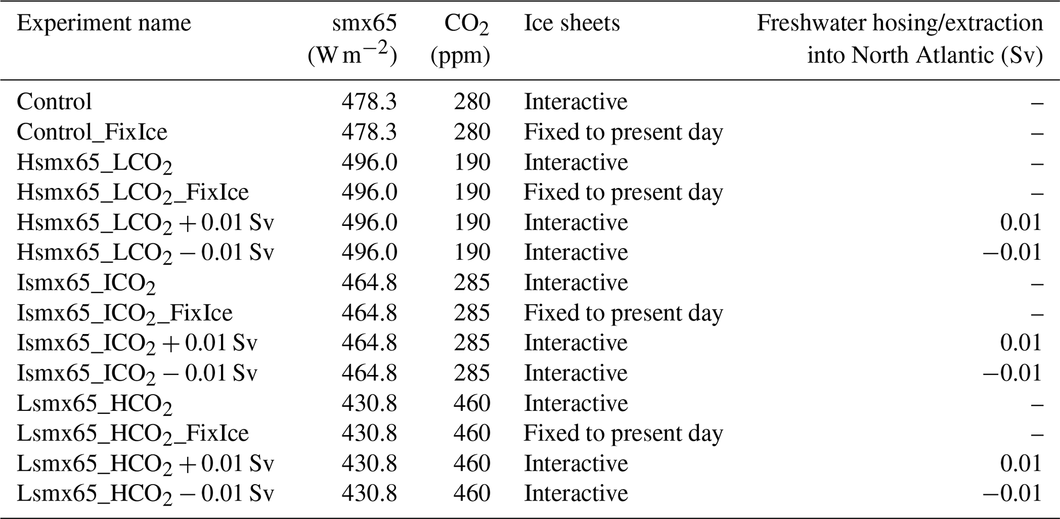
To validate the model suitability for tracing glacial inception bifurcation transitions, similarly to Ganopolski et al. (2016), we test the model performance against two paleoclimatic constraints. The first constraint is that, for a present-day orbital configuration and atmospheric CO₂ concentration of 280 ppm (named the Control simulation, Table 1), the model should not produce any substantial ice growth outside of Greenland. The second constraint is that, on the contrary, for the same 280 ppm level of atmospheric CO₂ concentration but an orbital configuration corresponding to the end of MIS11 (398 kyr BP), significant ice growth, indicative of glacial inception, should occur. Under the current model version these two constraints are met: after 100 kyr of simulation the NH ice volume totals, including the Greenland ice sheet, 8.3 $\mathrm{m}\mathrm{s}.\mathrm{l}.\mathrm{e}.$ for the present-day case and 21 $\mathrm{m}\mathrm{s}.\mathrm{l}.\mathrm{e}.$ for the MIS11 configuration.

Additional experiments with prescribed present-day ice sheets or applying freshwater hosing and extraction in the North Atlantic Ocean to alter AMOC strength are also conducted for selected orbital forcing–CO₂ configurations (Table 1).

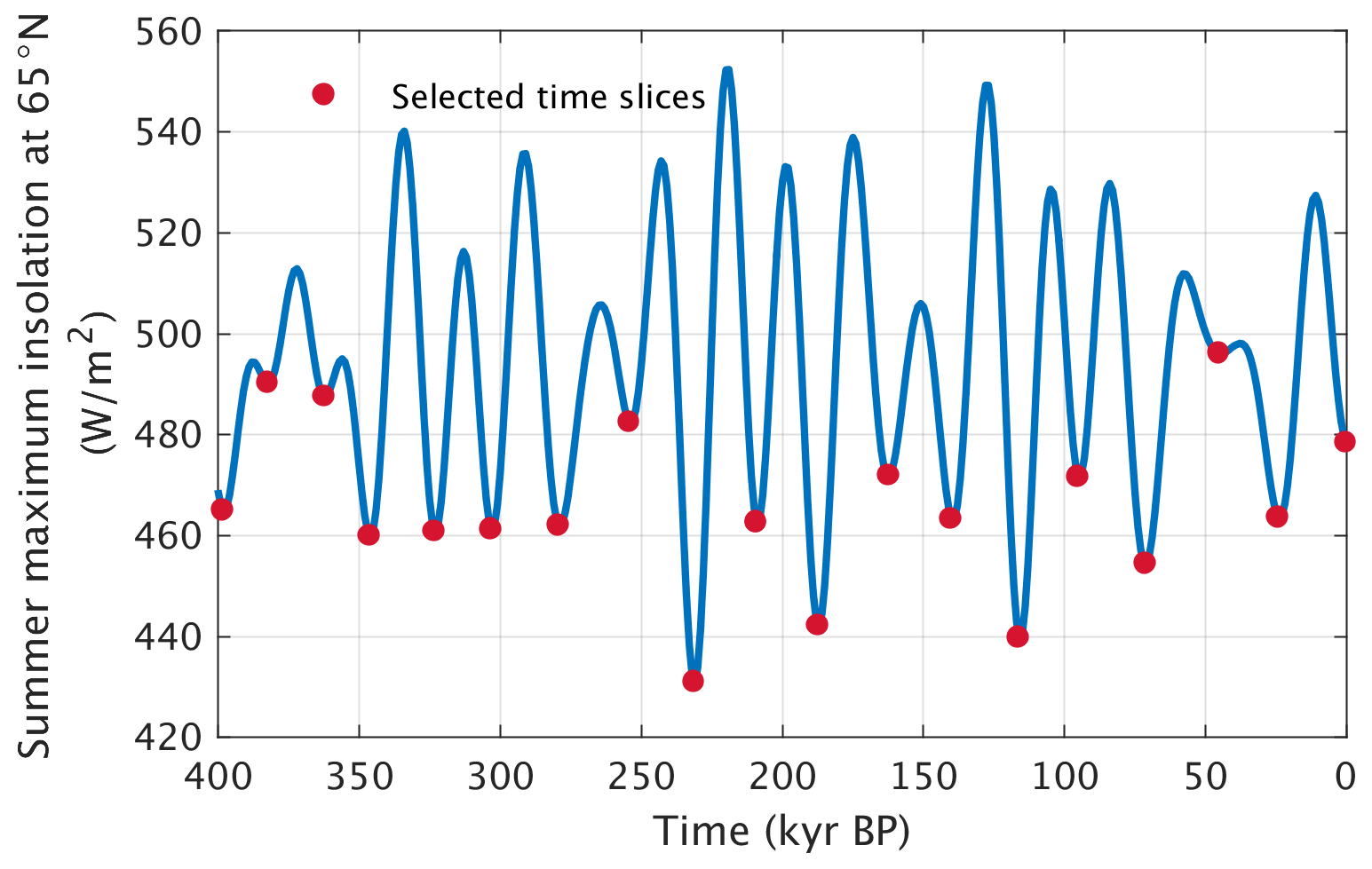
Figure 1 Summer maximum insolation at 65° N (smx65) in the period 400 kyr BP–present, computed using Laskar et al. (2004) data for Earth orbital parameters. Marked in red are all 19 local minima of the time series, whose orbital configurations are selected for the CLIMBER-X experiments.

Table 1 Summary of selected experiment configurations.

3 Results

3.1 Critical smx65–CO₂ relationship for triggering glacial inception

The usage of smx65 as a proxy for orbital forcing is common practice and considered a good metric for the analysis of glacial inception processes (Ganopolski et al., 2016; Paillard, 1998; Leloup and Paillard, 2022), as 65° N latitude coincides with the presence of land potentially capable of supporting the initial growth of ice sheets.

Considering smx65 to be an orbital forcing indicator, Fig. 2 shows the critical smx65–CO₂ combinations for triggering glacial inception in the 19 individual sets of experiments. Accounting for the fact that the radiative effect of CO₂ is logarithmic and that the temperature response to insolation is linear, we fit the data (via least squares) with curves of the shape

$$\begin{array}{}\text{(1)}& \mathrm{smx}{\mathrm{65}}_{\mathrm{cr}}=\mathit{\alpha }\ln {\displaystyle \frac{{\mathrm{CO}}_{\mathrm{2}}}{\mathrm{280}}}+\mathit{\beta }.\end{array}$$

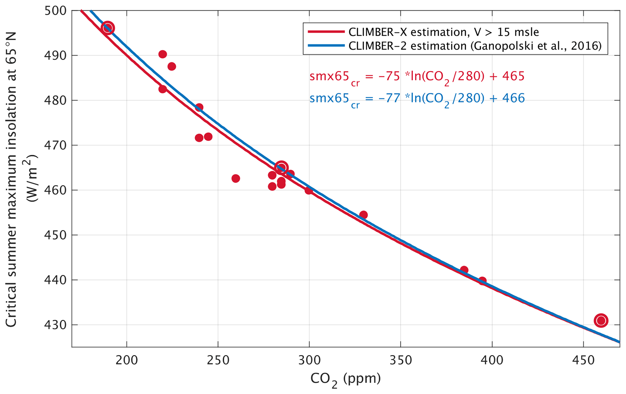
Figure 2 CLIMBER-X estimation of critical summer maximum insolation at 65° N (smx65) and CO₂ for triggering glacial inception at the threshold of 15 $\mathrm{m}\mathrm{s}.\mathrm{l}.\mathrm{e}.$ (red dots). The red line corresponds to the least-square fit following a logarithmic shape. The CLIMBER-2 estimation from Ganopolski et al. (2016) is depicted in blue. Big red circles indicate the experiments Hsmx65_LCO₂, Ismx65_ICO₂ and Lsmx65_HCO₂.

The least-squares fit of the data points produces values of α= −75 W m⁻² and β=465 W m⁻². The fit is good, with a coefficient of determination R²=0.95. The largest error in the fit is produced for an intermediate insolation case (462 W m⁻², corresponding to the minimum in summer solstice insolation at 209 ka), in which the difference between the least-squares fit and the CLIMBER-X result for the critical insolation is 8 W m⁻². This deviation from the best fit is explained by a very high obliquity at that time (see Sect. 3.3). The new CLIMBER-X estimation for α and β is very similar to the one generated with the CLIMBER-2 model and presented in Ganopolski et al. (2016). For that study the criterion for defining glacial inception was comparable (growth of the NH ice sheets of more than 13.5 $\mathrm{m}\mathrm{s}.\mathrm{l}.\mathrm{e}.$ was required), and the values for α and β were −77 and 466 W m⁻², respectively. The robustness of the estimated parameters of the critical insolation–CO₂ relationship is also supported by the theoretical analysis presented in Appendix A, where it is shown that for climate conditions similar to pre-industrial, the value of α is about −80 W m⁻². Moreover, the value derived from the results presented by Abe-Ouchi et al. (2013) is −83 W m⁻² (note that this number was not reported in Abe-Ouchi et al., 2013, but can be calculated from their Fig. 2). As was shown in Ganopolski et al. (2016), the value of β is reasonably well constrained by paleoclimate data since the critical insolation curve must pass between rather close insolation values corresponding to the end of MIS11 and present insolation. At the same time, paleo-data provide no constraint on the value of α. This is why, in Talento and Ganopolski (2021), we used a very conservative approach by accepting as “valid” any α values from the range −150 to 0 W m⁻²; i.e., we assumed relative uncertainties of up to 100 %. The results of the present study strongly indicate that the uncertainty is much smaller, likely not higher than 20 %. Such a reduction of the uncertainty range would also significantly reduce the uncertainties in the projections of the timing of future glaciations for different anthropogenic CO₂ emissions.

In order to better understand glacial inception at the critical insolation–CO₂ threshold and to evaluate similarities and differences for diverse insolation–CO₂ pairings, we select three experiments and analyze the temporal and spatial evolution of ice sheet growth. The three experiments (Hsmx65_LCO₂, Lsmx65_HCO₂ and Ismx65_ICO₂) correspond to either the highest, lowest or an intermediate value of the 19 smx65 time series local minima, respectively. In each experiment, the atmospheric CO₂ corresponds to the critical CO₂ for triggering glacial inception (Table 1). While, by definition, all three experiments Hsmx65_LCO₂, Lsmx65_HCO₂ and Ismx65_ICO₂ reach at least 15 $\mathrm{m}\mathrm{s}.\mathrm{l}.\mathrm{e}.$ NH ice volume at some point during the simulation, they do it with different temporal and spatial dynamics (Figs. 3 and 4).

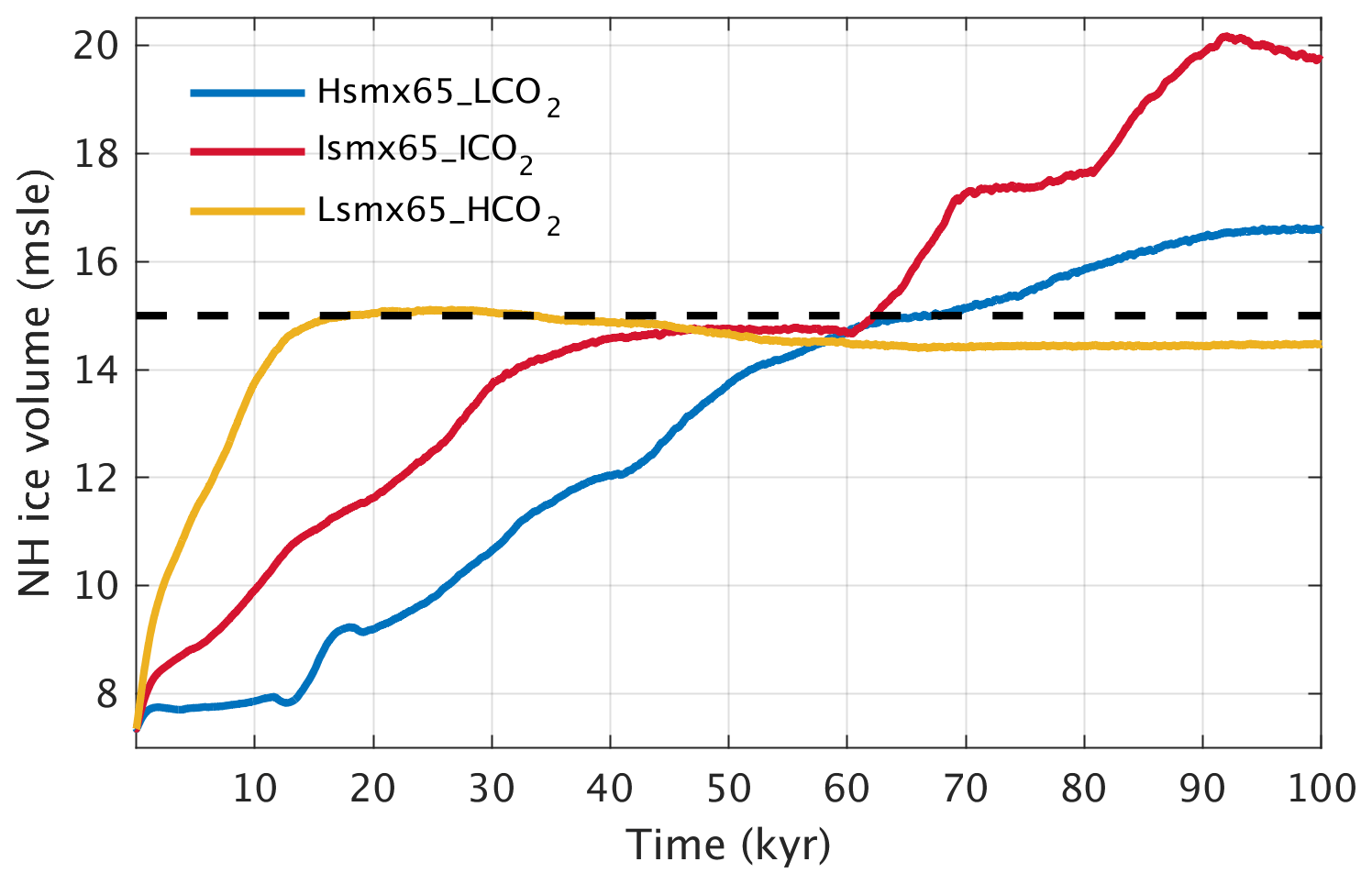
Figure 3 NH ice volume (m s.l.e.) temporal evolution at the critical combination of smx65 and CO₂ for triggering glacial inception (threshold 15 $\mathrm{m}\mathrm{s}.\mathrm{l}.\mathrm{e}.$ level, dashed line) for three selected experiments (see Table 1).

For the experiment Hsmx65_LCO₂ (smx65 =496 W m⁻² and CO₂ = 190 ppm) the NH ice volume time series crosses the 15 $\mathrm{m}\mathrm{s}.\mathrm{l}.\mathrm{e}.$ threshold 67 kyr into the simulation and reaches a quasi-equilibrium value of 16.6 $\mathrm{m}\mathrm{s}.\mathrm{l}.\mathrm{e}.$ only after 90 kyr (Fig. 3). At the moment of crossing the glacial inception threshold (15 $\mathrm{m}\mathrm{s}.\mathrm{l}.\mathrm{e}.$), the ice sheets have significantly developed outside of Greenland over Iceland, Svalbard, Novaya Zemlya and the Scandinavian Peninsula as well as in North America, north of Hudson Bay, from 90 to 70° W (Fig. 4a). The Scandinavian ice sheet development is aided by a weak AMOC (Fig. 5) and subsequent weakened meridional heat transport from the tropics towards that region. The AMOC reaches quasi-equilibrium conditions in the second half of the simulation, with a maximum magnitude of ∼ 16 Sv. At the threshold crossing time, the AMOC is weak and shallow (Fig. 6a) and deep convection in the North Atlantic Ocean only occurs in the Norwegian Sea (Fig. 6d).

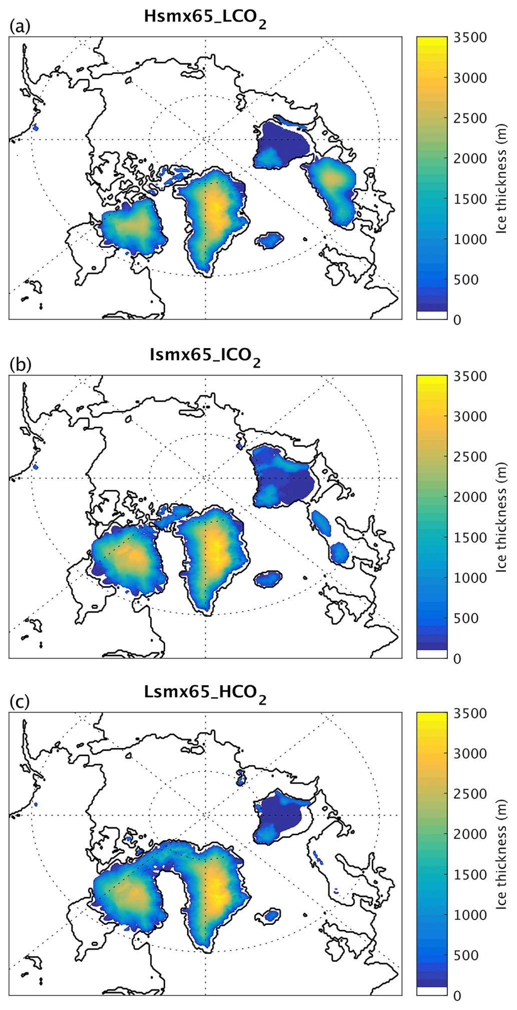
Figure 4 Ice thickness (a–c) for Hsmx65_LCO₂, Ismx65_ICO₂ and Lsmx65_HCO₂ at the time when each experiment reaches the 15 $\mathrm{m}\mathrm{s}.\mathrm{l}.\mathrm{e}.$ threshold.

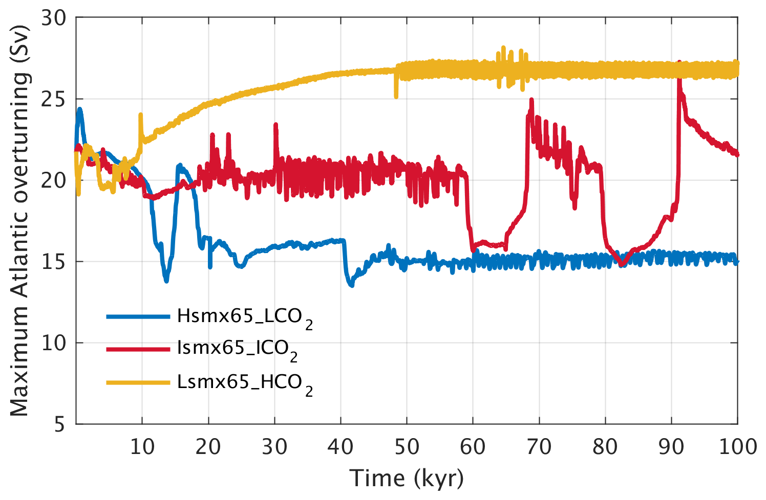
Figure 5 Maximum Atlantic overturning (Sv) temporal evolution at the critical combination of smx65 and CO₂ for triggering glacial inception (threshold 15 $\mathrm{m}\mathrm{s}.\mathrm{l}.\mathrm{e}.$ level) for three selected experiments (see Table 1).

In the experiment Ismx65_ICO₂ (smx65 =464.8 W m⁻² and CO₂ = 285 ppm) the NH ice volume time series shows a faster increasing rate at the start of the experiment than the Hsmx65_LCO₂ experiment but stagnates at 14.5 $\mathrm{m}\mathrm{s}.\mathrm{l}.\mathrm{e}.$ between 40 and 60 kyr of simulation. At 60 kyr of simulation, the time series shows an abrupt increase, crossing the 15 $\mathrm{m}\mathrm{s}.\mathrm{l}.\mathrm{e}.$ threshold at 63 kyr. After that, the time series stagnates again at 17.5 $\mathrm{m}\mathrm{s}.\mathrm{l}.\mathrm{e}.$ before showing another abrupt increase towards the end of the simulated period. In the 100 kyr of simulation, quasi-stationary conditions are not reached (Fig. 3). In this experiment, the AMOC is unstable and oscillates between ∼ 25 and ∼ 16 Sv (Fig. 5). It should be noted that the timescale of these simulated oscillations is distorted by the climate acceleration factor. The AMOC weakening episodes precede the abrupt NH ice volume growth and are thus likely triggers. At the moment when the NH ice volume is 15 $\mathrm{m}\mathrm{s}.\mathrm{l}.\mathrm{e}.$, ice sheets cover the north of Hudson Bay from 100 to 70° W (covering almost the totality of Baffin Island), and there is full ice coverage of Iceland, Svalbard and Novaya Zemlya and partial ice coverage of Scandinavia (Fig. 4c). The moderate ice growth over Scandinavia is related to the AMOC weakening episodes (Fig. 5) and the consequential decreased heat transport from the tropics, as such ice growth is inhibited in simulations with a stable AMOC (see Sect. 3.2 with extraction simulation Ismx65_ICO₂ − 0.01 Sv). At the time of the 15 $\mathrm{m}\mathrm{s}.\mathrm{l}.\mathrm{e}.$ crossing, the Atlantic overturning circulation penetrates to ∼ 3000 m of depth and deep-water formation does not occur in the Labrador Sea and south of Greenland (Fig. 6b, e).

The Lsmx65_HCO₂ experiment (smx65 =430.8 W m⁻² and CO₂ = 460 ppm) shows the fastest NH ice volume time series increase at the start of the simulation, crossing the 15 $\mathrm{m}\mathrm{s}.\mathrm{l}.\mathrm{e}.$ threshold after only 18 kyr of simulation. After that, the ice volume slightly decreases, stabilizing at 14.5 $\mathrm{m}\mathrm{s}.\mathrm{l}.\mathrm{e}.$ (Fig. 3). At the moment of crossing of the threshold, the ice sheet coverage over North America is larger than in the other two experiments, while no ice sheet develops over Scandinavia (Fig. 4c). For this case, the AMOC reaches equilibrium with a maximum strength of 27 Sv in the second half of the simulation (Fig. 5). Deep convection is widespread in the North Atlantic, occurring over the Labrador Sea, south of Greenland and the Norwegian Sea (Fig. 6f). The Atlantic overturning circulation reaches depths of 4000 m (Fig. 6c).

From these experiments it is clear that the timescales involved with glacial development in the vicinity of the glacial inception bifurcation point are extremely long and that even 100 kyr of simulation might not be enough to reach stationary conditions. It is also clear that, in CLIMBER-X, glacial inception can occur for different AMOC configurations. The spatial patterns of glaciation are different and related to the AMOC intensity, with a weak AMOC transporting less heat from the tropics towards Scandinavia and facilitating ice growth there. We see that in quasi-equilibrium conditions higher atmospheric CO₂ concentrations produce a stronger AMOC in CLIMBER-X. This was also observed in CLIMBER-2 (Bouttes et al., 2012; Gottschalk et al., 2019) and general circulation models, starting from Stouffer and Manabe (2003), who found AMOC strengthening under doubling and quadrupling of CO₂ and significant AMOC weakening under CO₂ halving in multimillennial simulations. Recently, Bonan et al. (2022) described the AMOC response to instantaneous CO₂ quadrupling in several state-of-the-art climate models. Mots of the runs were not long enough, and the AMOC continues to evolve through the runs, but at least in one model (CESM1), the AMOC is appreciably stronger under CO₂ quadrupling. For a lower CO₂ concentration, there are two systematic studies (Oka et al., 2012; Galbraith and de Lavergne, 2019) where it has been shown that global cooling causes a weakening of the AMOC.

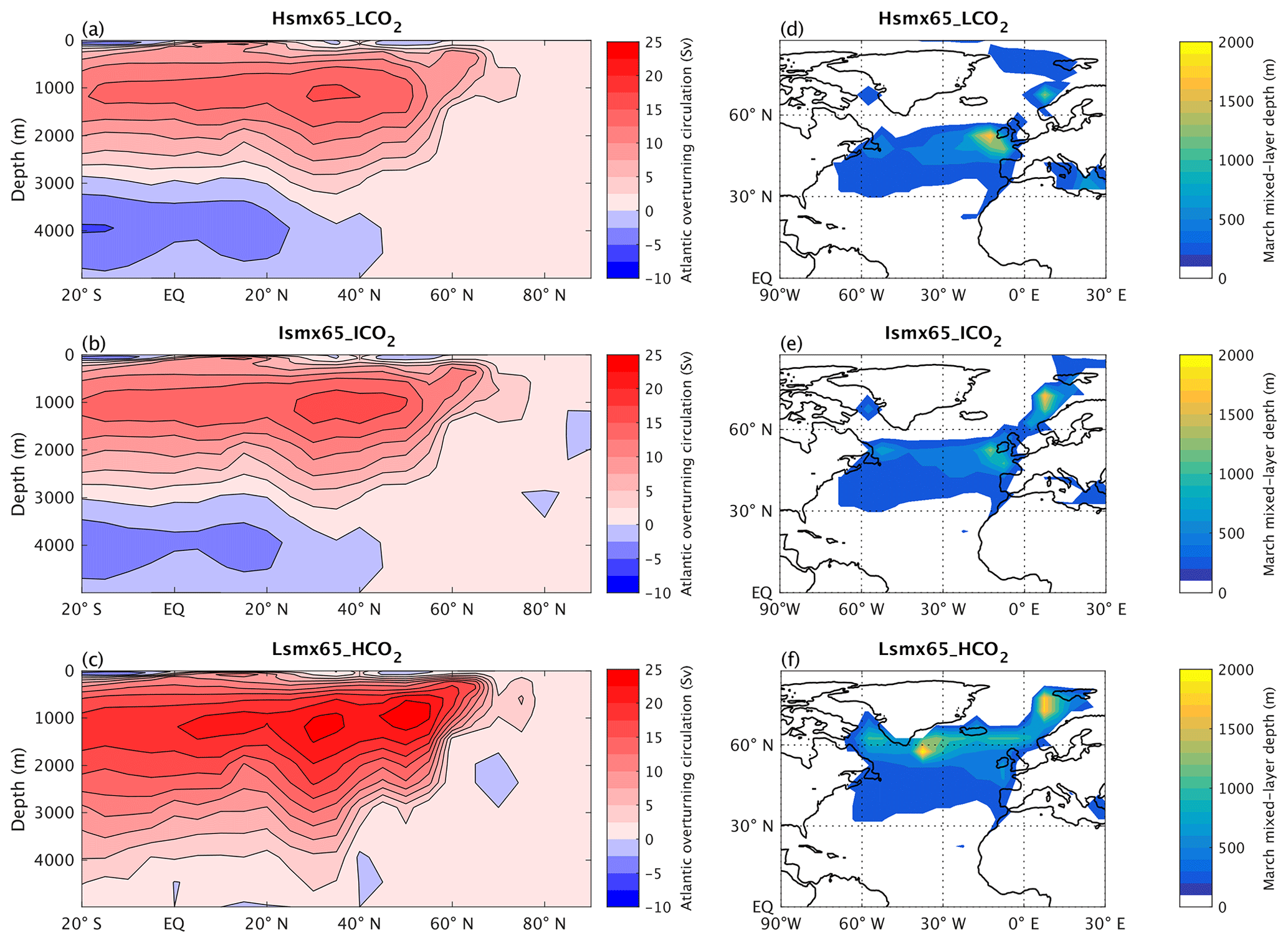
Figure 6 Annual mean Atlantic Ocean meridional overturning circulation streamfunction (a–c) and maximum (March) mixed layer depth (d–f) for the experiments Hsmx65_LCO₂, Ismx65_ICO₂ and Lsmx65_HCO₂ at the time when each experiment reaches the 15 $\mathrm{m}\mathrm{s}.\mathrm{l}.\mathrm{e}.$ threshold.

To get a better understanding on how different spatial patterns of ice growth arise with different combination of insolation and CO₂, we analyze the climatic conditions leading to the ice development. Figure 7 displays the annual mean surface mass balance (SMB) anomalies with respect to Control at the moment when the simulations reach the 15 $\mathrm{m}\mathrm{s}.\mathrm{l}.\mathrm{e}.$ of NH ice volume. For the three experiments, positive SMB anomalies with respect to Control are found over Greenland and over Baffin Island, the anomalies being larger in magnitude for the Lsmx65_HCO₂ case. For the Hsmx65_LCO₂ experiment, the largest positive anomalies occur over the Scandinavian Peninsula.

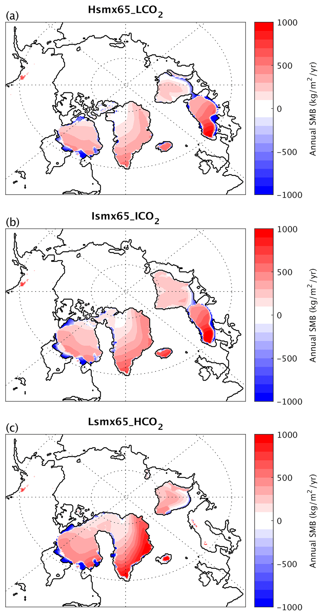
Figure 7 Annual surface mass balance anomaly with respect to Control for the experiments Hsmx65_LCO₂, Ismx65_ICO₂ and Lsmx65_HCO₂ (a–c), respectively, at the time when each experiment reaches the 15 $\mathrm{m}\mathrm{s}.\mathrm{l}.\mathrm{e}.$ threshold. Continental and ice sheet margins are show in black.

Given the fact that surface temperature and precipitation fields might be directly impacted by the presence of an ice sheet, we generate auxiliary experiments in which the conditions are the same as in Hsmx65_LCO₂, Ismx65_ICO₂ and Lsmx65_HCO₂ but without interactive ice sheets (i.e., the ice sheets remain constant and equal to the initial present-day conditions; Table 1) and denote them with an additional FixIce label.

Boreal summer (June–August; JJA) 2 m temperature and annual precipitation anomalies with respect to Control in simulations without interactive ice sheets for the NH between 120° W and 60° E are displayed in Fig. 8. The largest temperature differences between experiments are seen over the northern North Atlantic and are related to the differences in AMOC strength and related northward oceanic heat transport. The AMOC is the weakest in Hsmx65_LCO₂_FixIce, and as a result, Scandinavia is colder in this experiment by 2–4 °C than in the Control experiment. This explains why the ice sheets developed in Scandinavia in Hsmx65_LCO₂ but not in Lsmx65_HCO₂. Over northern North America, temperatures are rather similar in all experiments, which is explained by the fact that summer temperatures are the main factor controlling the mass balance of ice sheets. Still, temperatures in Hsmx65_LCO₂ are lower by ca. 2 °C than in Lsmx65_HCO₂_FixIce. The reason why glacial inception requires lower temperatures in experiments with higher insolation is straightforward. Unlike CO₂, insolation affects the surface mass balance of ice sheets not only through temperature but also directly through absorbed shortwave radiation (e.g., Robinson et al., 2010). This is why, to compensate for the effect of higher insolation on surface ice sheet melt in the experiment Hsmx65_LCO₂, summer temperatures should be lower than in the experiments where glacial inception is simulated under lower summer insolation.

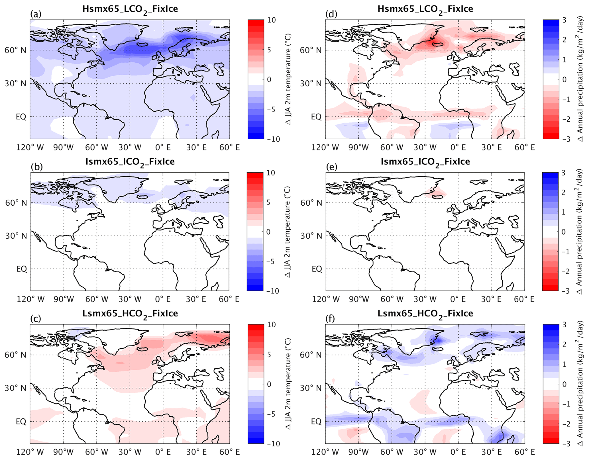
Figure 8 Summer (JJA) temperature anomalies (a–c) and annual precipitation anomalies (d–f) with respect to Control_FixIce for experiments Hsmx65_LCO₂_FixIce, Ismx65_ICO₂_FixIce and Lsmx65_CO₂_FixIce. Control continental margins (present-day conditions) are shown in black.

Annual precipitation anomalies relative to Control shown in Fig. 8d–f also mostly reflect changes in AMOC, although globally there is more precipitation under a higher CO₂ level. Over Scandinavia, precipitation changes counteract temperature changes, but the effect of temperature is dominant. This is why, in spite of significantly lower annual precipitation, the ice sheet in Scandinavia grows in the experiment Hsmx65_LCO₂ but not in Lsmx65_HCO₂. Precipitation differences in northern North America are small.

In general, a comparison of these three experiments shows that summer climate conditions corresponding to the initiation of glaciation are similar in North America despite very different insolation and CO₂ in these experiments. This explains rather similar patterns of initial ice sheet growth in North America. Climate conditions are more different in Scandinavia, and this is why glaciation develops here simultaneously with glaciation in North America only under sufficiently low CO₂.

3.2 Role of AMOC change in glacial inception

As shown above, the AMOC state is different for different combinations of insolation–CO₂ close to the glacial inception limit (Fig. 6a–c). The question therefore arises of what role the AMOC plays for glacial inception. To explore the relative importance of the AMOC state compared to the summer insolation and the atmospheric CO₂ concentration in shaping the conditions for glacial inception, we have performed additional simulations in order to separate the contribution of the different factors. For that we have taken the extreme cases, Hsmx65_LCO₂ and Lsmx65_HCO₂, and run three sets of model simulations with prescribed present-day ice sheets:

• present-day orbital configuration with CO₂ concentration corresponding to HCO₂ and LCO₂,

• pre-industrial CO₂ concentration with orbital configuration corresponding to Hsmx65 and Lsmx65,

• pre-industrial CO₂ concentration and orbital configuration with and without 0.1 Sv freshwater hosing in the North Atlantic between 50–70° N to get two states with weak and strong AMOC (∼ 10 Sv difference roughly corresponding to the difference between Hsmx65_LCO₂ and Lsmx65_HCO₂ experiments) under the same background climate conditions.

These three sets of two simulations each allow separating the effect of atmospheric CO₂, summer insolation and AMOC state on the summer temperature in the NH. The results clearly show that summer temperatures at the locations where the ice sheets start to grow during glacial inceptions (i.e., Scandinavia and northeastern Canada) are much more sensitive to CO₂ and orbital forcing than to changes in the AMOC (Fig. 9). The AMOC state has a generally larger impact on summer temperatures over Scandinavia (Fig. 9c), at least partly explaining why the inception patterns show the largest differences there (Fig. 4). It has to be noted that changes in CO₂ and insolation also affect the AMOC. In particular, the AMOC is stronger by 9 Sv in the experiment with high CO₂ compared to low CO₂ and by 3 Sv in experiments with high insolation compared to low insolation. However, as seen from Fig. 9c, these changes can contribute only a little to the direct effect of CO₂ (Fig. 9a) and insolation (Fig. 9b). Thus, at the potential locations of glacial inception, AMOC changes provide a positive, but not very strong, feedback to both primary forcings.

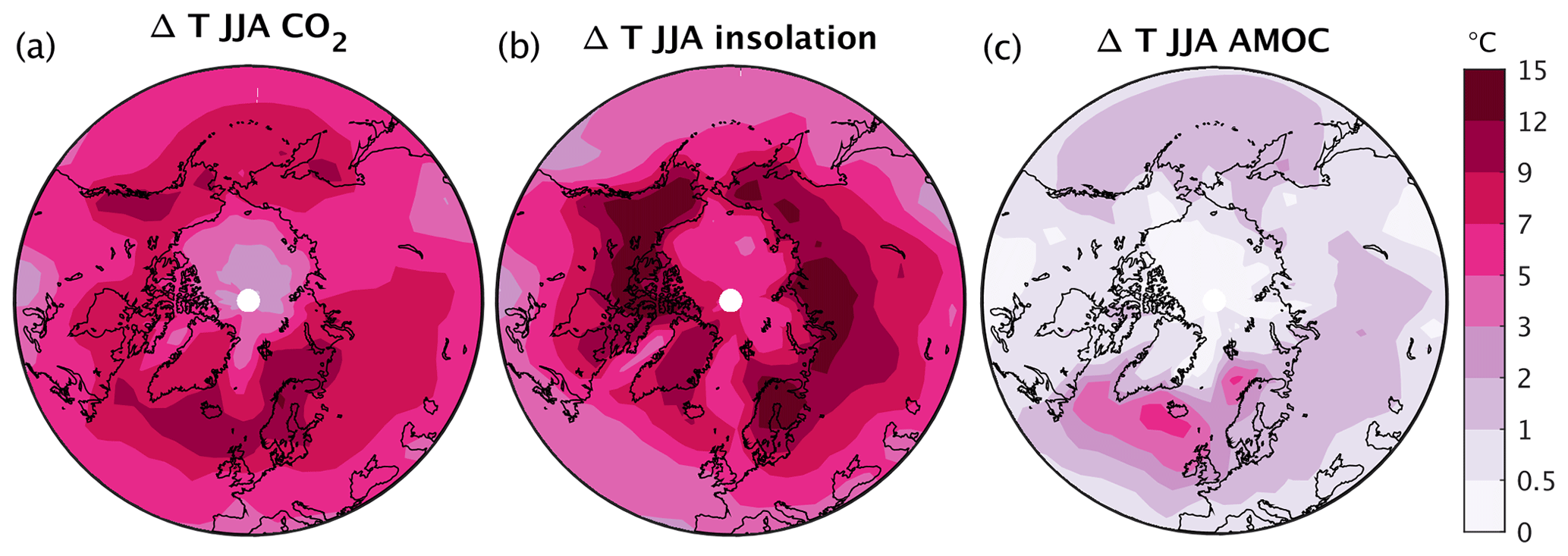
Figure 9 Summer (JJA) temperature differences due to (a) CO₂ (HCO₂–LCO₂), (b) insolation (Hsmx65–Lsmx65) and (c) AMOC state (strong–weak).

To further investigate the role of AMOC strength change at the glacial inception bifurcation limits, we produce a series of water hosing and extraction experiments (Table 1). The freshwater forcing is applied in the North Atlantic Ocean between 50 and 70° N and compensated for over the tropical (30° S–30° N) Pacific Ocean to prevent a global salinity drift. The magnitude of the freshwater flux is 0.01 Sv, either positive (added freshwater, leading to a weakening of AMOC) or negative (extracted freshwater, leading to a strengthening of AMOC). The hosing and extraction forcing is applied for the whole duration of the experiments. Note that 0.01 Sv is a very small value compared to a typical stability threshold for the AMOC in the CLIMBER-X model (Willeit et al., 2022).

The freshwater extraction produces less NH ice sheet volume in all three cases (Fig. 10). In particular, in the experiments Hsmx65_LCO₂ and Ismx65_ICO₂ the extraction in enough to prevent the NH ice volume from crossing the 15 $\mathrm{m}\mathrm{s}.\mathrm{l}.\mathrm{e}.$ threshold used for the definition of glacial inception. In opposition, the freshwater hosing flux produces in all three cases faster and larger ice growth in the NH. The largest change in terms of NH ice volume is produced for Ismx65_ICO₂, reaching a magnitude of ∼ 150 $\mathrm{m}\mathrm{s}.\mathrm{l}.\mathrm{e}$. In this case, the freshwater hosing flux produces the largest AMOC weakening of all three experiments and even an almost complete AMOC shutdown between 50 and 80 kyr of the simulation (Fig. 11).

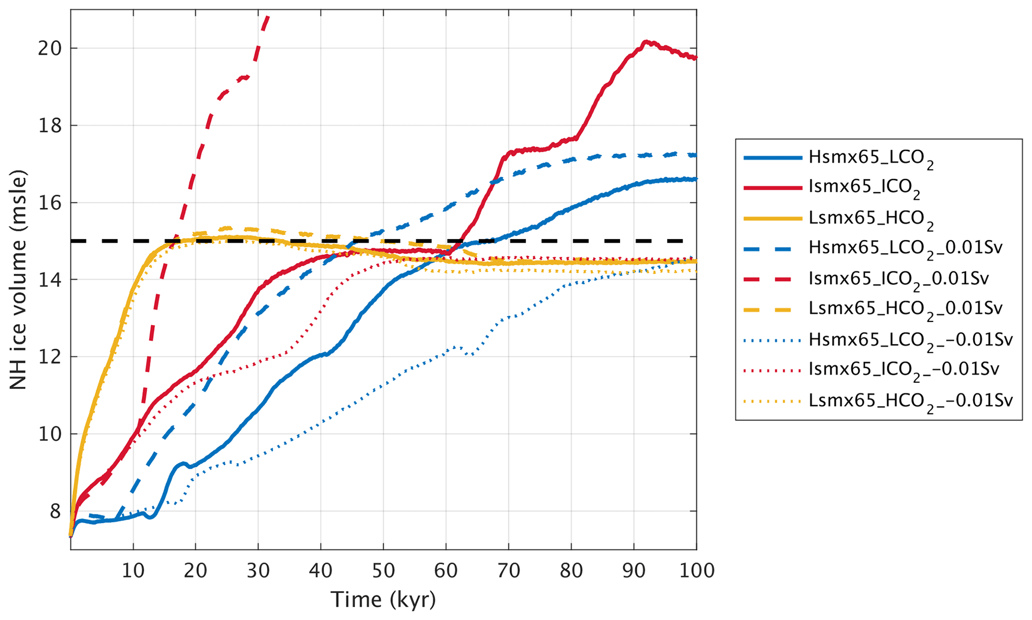
Figure 10 NH ice volume (m s.l.e.) temporal evolution in water hosing and extraction experiments (Table 1).

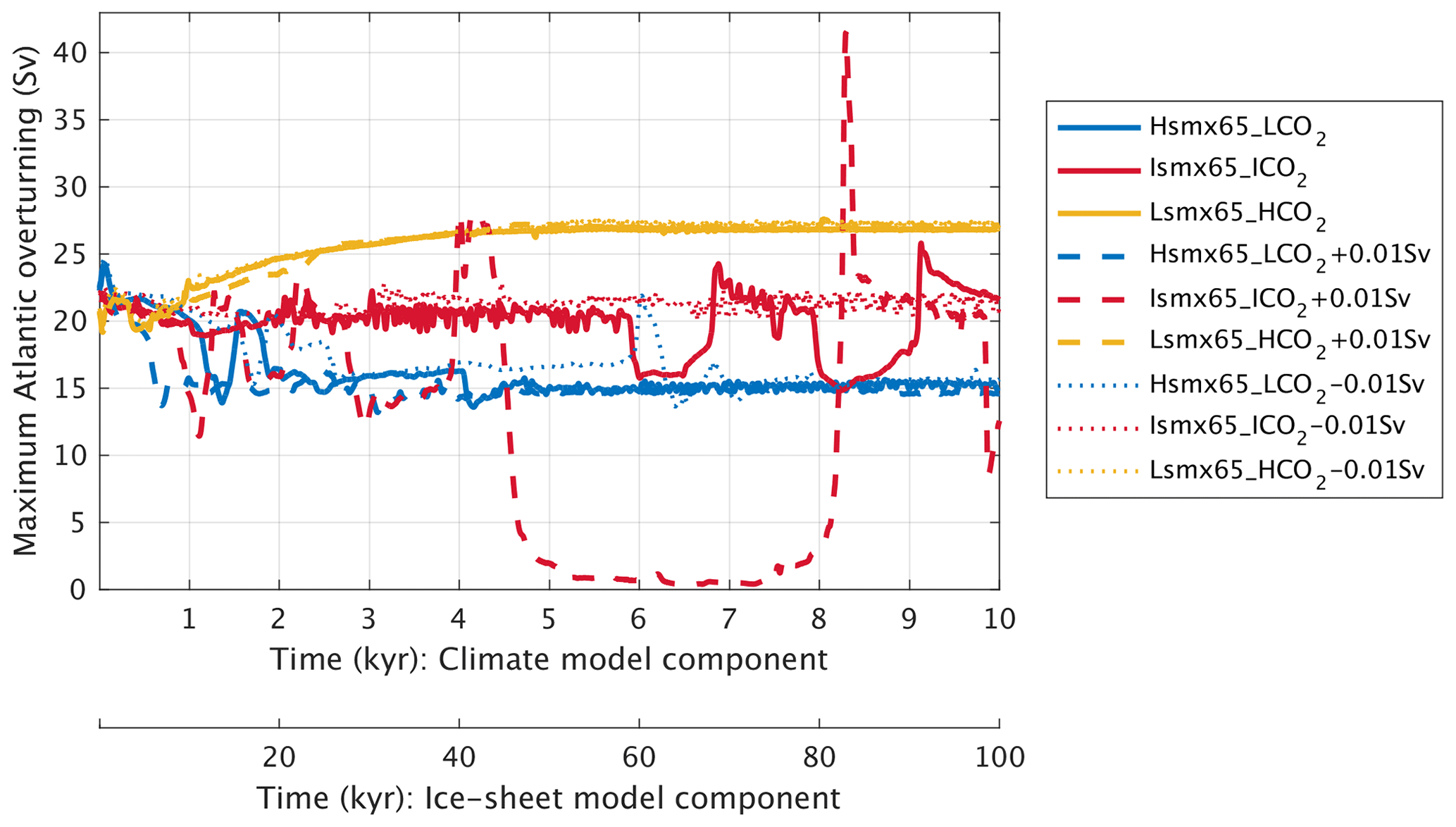
Figure 11 Maximum Atlantic overturning (Sv) temporal evolution in water hosing and extraction experiments (Table 1).

This set of hosing experiments shows that the AMOC (in particular its stability) plays a role in triggering glacial inception and the rate of ice growth. In general, the weaker the AMOC the larger and faster the development of the NH ice sheets for a given insolation–CO₂ pairing.

3.3 Suitability of smx65 as a proxy for orbital forcing

The usage of smx65 as a proxy for orbital forcing in tracing the glacial inception bifurcation is justified by the relevance of 65° N latitude for the development of ice sheets (Ganopolski, 2024). However, as with any simple metric for such a complex phenomenon as the influence of orbital forcing on Earth climate, it cannot be perfect. This is why it is not surprising that although most of the points in Fig. 2 are located very close to the proposed logarithmic curves, several deviate more significantly, for example the point corresponding to insolation at 209 ka, as it was discussed above.

To evaluate the possibility of improving the proxy for orbital forcing, we separate the smx65 time series into its obliquity and precessional components (as in Jackson and Broccoli, 2003). The decomposition is done via a least-squares fit to the data of the last 400 kyr, expressing the smx65 time series in the form

$$\begin{array}{}\text{(2)}& \mathrm{smx}\mathrm{65}=a_{\mathrm{0}}+a_{\mathrm{1}}\cdot \mathrm{ecc}\cdot \sin \mathit{\omega }+a_{\mathrm{2}}\cdot (\mathrm{obl}-\stackrel{\mathrm{‾}}{\mathrm{obl}}),\end{array}$$

with ecc, ω and obl denoting eccentricity, longitude of perihelion and obliquity, respectively; coefficients a₀, a₁ and a₂ are derived from the least-squares fit and the overbar indicates time averaging. The precessional (smx65_p) and obliquity (smx65_o) components are defined as

$$\begin{array}{}\text{(3)}& {\displaystyle }\mathrm{smx}{\mathrm{65}}_{\mathrm{p}}=a_{\mathrm{0}}+a_{\mathrm{1}}\cdot \mathrm{ecc}\cdot \sin \mathit{\omega }.\text{(4)}& {\displaystyle }\mathrm{smx}{\mathrm{65}}_{\mathrm{o}}=a_{\mathrm{2}}\cdot (\mathrm{obl}-\stackrel{\mathrm{‾}}{\mathrm{obl}}).\end{array}$$

We analyze different linear combinations of smx65_p and smx65_o as alternative proxies for orbital forcing. We wish to find γ, which maximizes the goodness of fit (R² coefficient of determination) between the logarithm of critical CO₂ and the generalized proxy for summer insolation in the form smx65_p+γsmx65_o.

Any value of γ between 1 and 2 yields an extremely good fit (R² higher than 0.95), and thus the quantities smx65_p+γsmx65_o for those values of γ are good proxies for orbital forcing (Fig. 12). Values of γ lower than 1, in which the contribution of obliquity is considered relatively less important than that of precession, are not optimal proxies. Similarly, values of γ higher than 2 (i.e., the obliquity contribution is weighted more than the precessional one) are also not adequate. The best fit is found for γ≈1.3. Although this fit is only marginally better than for γ=1, corresponding to smx65, and thus of little importance for the main results presented in this paper, it still can help to explain some deviations of individual results from the logarithmic curve. Indeed, as was discussed in Ganopolski (2024), the smx65 metric contains the smallest contribution of obliquity compared to other proposed proxies for orbital forcing. The results of the analysis presented above suggest that the relative contribution of obliquity is underestimated in smx65 by ca. 30 %. Since the amplitude of obliquity contribution to smx65 is only about 15 W m⁻², the generalized proxy for summer insolation for γ=1.3 would not deviate from smx65 by more than 5 W m⁻², which is very small compared to smx65 values. However, it has an implication for the “outlier” in Fig. 2 corresponding to insolation at 209 ka, when obliquity was close to its maximum value during the entire past 800 kyr. The correction upwards by 5 W m⁻² would bring the point corresponding to 209 ka insolation much closer to the logarithmic curve.

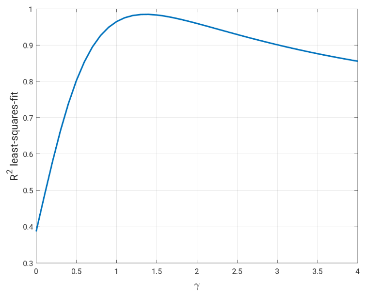
Figure 12 Goodness of fit (R² coefficient of determination) derived from the least-squares fit between ln (CO_2,critical) and smx65_p+γsmx65_o as a function of γ, considering CO₂ values critical for glacial inception at the 15 $\mathrm{m}\mathrm{s}.\mathrm{l}.\mathrm{e}.$ level.

4 Summary and conclusions

We used the recently developed EMIC CLIMBER-X to produce a new estimation of the critical insolation–CO₂ relationship for triggering glacial inception. The use of CLIMBER-X for tracing the glacial inception bifurcation constitutes a further development from previous attempts produced with the coarser-resolution and simpler CLIMBER-2 model (Ganopolski et al., 2016; Archer and Ganopolski, 2005).

The study is based on sets of equilibrium experiments in which the orbital parameters and atmospheric CO₂ concentration are kept constant in time. The sets are based on orbital configurations corresponding to all the local minima of summer maximum insolation at 65° N (smx65) of the last 400 kyr. Therefore, our experiments reflect a diverse arrangement of orbital parameters in configurations potentially favorable for glacial inception. The estimation of the glacial inception bifurcation is done within a 5 ppm resolution in the CO₂ phase space.

The new estimation of the critical insolation–CO₂ relationship for triggering glacial inception follows a logarithmic dependence, explained by the logarithmic shape of the radiative forcing of CO₂. When considering that glacial inception occurs if the NH ice volume develops at least 15 $\mathrm{m}\mathrm{s}.\mathrm{l}.\mathrm{e}.$, the new CLIMBER-X estimation for the critical summer maximum insolation at 65° N and CO₂ relationship is

$$\begin{array}{}\text{(5)}& \mathrm{smx}{\mathrm{65}}_{\mathrm{cr}}=-\mathrm{75}\cdot \ln {\displaystyle \frac{{\mathrm{CO}}_{\mathrm{2}}}{\mathrm{280}}}+\mathrm{465}.\end{array}$$

This new estimation is close to the one produced with CLIMBER-2 in Ganopolski et al. (2016), who used a similar threshold for NH ice volume. Moreover, we showed that the summer maximum insolation at 65° N is a skillful single metric for tracing the glacial inception bifurcation.

We also showed that the temporal and spatial patterns of glacial inception depend on the combination of insolation and critical CO₂ concentration. In all simulations of glacial inception, ice sheets developed north of Hudson Bay in North America, as well as in Iceland and Svalbard. Considerable ice growth over the Scandinavian Peninsula is only observed in experiments in which the Atlantic Meridional Overturning Circulation (AMOC) significantly weakens, which occurs in either low-CO₂ cases (stable weak AMOC) or intermediate-CO₂ situations (unstable AMOC with substantial weakening episodes). In general, the lower the CO₂, the weaker the AMOC and, thus, the weaker the heat transport from the tropics towards European high latitudes, facilitating the Scandinavian ice sheet development. The time needed for reaching the glacial inception bifurcation threshold varies between 18 000 and almost 100 000 years, highlighting the long timescales of the climate–cryosphere system at the bifurcation limit.

Appendix A: Theoretical derivation of the critical insolation–CO₂ relationship

To derive the critical insolation–CO₂ relationship for triggering glacial inception, we consider the surface energy balance of snow cover at the location where the nucleation of the northern continental ice sheet begins during glacial inceptions. Important assumptions are that

• this location remains the same for the different combinations of insolation and CO₂ and that

• glacial inception begins from the formation of extensive perennial snowfields rather than from the spreading of glaciers from high mountains.

Both these assumptions are consistent with the results of our model simulations. Surface daily mass balance of the snowpack during the melt season is described by the following equation:

$$\begin{array}{}\text{(A1)}& S_{\mathrm{abs}}+R_{\downarrow }-R_{\uparrow }+H=ML,\end{array}$$

where S_abs is the absorbed shortwave radiation, R_↓ is the downward longwave radiation flux near the Earth's surface, R_↑ is the longwave radiation emitted by the snow surface, H is the sensible heat flux (positive downward), M is the snowmelt rate in $\mathrm{kg}{\mathrm{m}}^{-\mathrm{2}}{\mathrm{s}}^{-\mathrm{1}}$ and L is the latent heat of fusion. Surface latent heat flux can be neglected during the melt season, as it is an order of magnitude smaller than shortwave and longwave radiation fluxes (e.g., Ettema et al., 2010). Since we consider only the period of snowmelt, surface temperature during this period is 0 °C. In this case, the terms on the left-hand side of Eq. (A1) can be expressed as follows:

$$\begin{array}{}\text{(A2)}& {\displaystyle }{S}_{\mathrm{abs}}=S(\mathrm{1}-{\mathit{\alpha }}_{\mathrm{s}})\mathit{\tau },\text{(A3)}& {\displaystyle }{R}_{\downarrow }=F\left(\mathrm{0}\right)+\mathit{\beta }T,\text{(A4)}& {\displaystyle }{R}_{\uparrow }=\mathit{ϵ}\mathit{\sigma }{T}_{\mathrm{0}}^{\mathrm{4}},\text{(A5)}& {\displaystyle }H=\mathit{\gamma }T,\end{array}$$

where T is the surface air temperature (in °C), S is the insolation at the top of the atmosphere, α_s is the surface albedo, τ is the atmospheric transmissivity, F(0) is the downward longwave radiation for a surface air temperature of 0 °C in W m⁻², T₀=273.15 K, $\mathit{\sigma }=\mathrm{5.67}\times {\mathrm{10}}^{-\mathrm{8}}$ $\mathrm{W}{\mathrm{m}}^{-\mathrm{2}}{\mathrm{K}}^{-\mathrm{4}}$ is the Stefan–Boltzmann constant, ϵ≈ 1 is the snow emissivity for longwave radiation, and α and β are empirical parameters. In the nucleation center of glacial inception (northern Canada and Baffin Island), the melt season is only about 2 months and approximately coincides with the period of positive air temperatures. This allows us to make further simplifications when integrating Eq. (A1) over the melt season after substituting Eqs. (A2), (A3), (A4) and (A5):

$$\begin{array}{}\text{(A6)}& \stackrel{\mathrm{‾}}{S}(\mathrm{1}-{\mathit{\alpha }}_{\mathrm{s}})\mathit{\tau }+F\left(\mathrm{0}\right)+\mathit{\beta }\stackrel{\mathrm{‾}}{T}-\mathit{\sigma }{T}_{\mathrm{0}}^{\mathrm{4}}+\mathit{\gamma }\stackrel{\mathrm{‾}}{T}=\stackrel{\mathrm{‾}}{M}L,\end{array}$$

where $\stackrel{\mathrm{‾}}{T}$ is the surface air temperature, $\stackrel{\mathrm{‾}}{S}$ is daily insolation and $\stackrel{\mathrm{‾}}{M}$ is snowmelt, all averaged over the melt season. Assuming that the duration of the melt season at the location of glacial inception is about 2 months (which is similar to present climate conditions in the area where glacial inception is simulated in CLIMBER-X), the seasonal surface air temperature evolution can be approximated by a sinusoidal function with zero air temperatures at the beginning and end of the melt season and the average insolation and temperature can be expressed through their maximum annual values as

$$\begin{array}{}\text{(A7)}& {\displaystyle }\stackrel{\mathrm{‾}}{S}=k_{\mathrm{S}}\mathrm{smx}\mathrm{65},\text{(A8)}& {\displaystyle }\stackrel{\mathrm{‾}}{T}=k_{\mathrm{T}}{T}_{\max },\end{array}$$

where k_S≈ 0.9 and k_T≈ 0.7 (see Fig. A1). Maximum summer air temperature is parameterized as

$$\begin{array}{}\text{(A9)}& T_{\max }=T_{\max }^{*}+\mathit{\delta }\ln {\displaystyle \frac{{\mathrm{CO}}_{\mathrm{2}}}{{\mathrm{CO}}_{{\mathrm{2}}_{\mathrm{0}}}}}+\mathit{\mu }\cdot (\mathrm{smx}\mathrm{65}-\mathrm{smx}{\mathrm{65}}^{*}),\end{array}$$

where $T_{\max }^{*}$ is the maximum summer temperature at the location of glacial inception for pre-industrial conditions, namely for CO₂ = CO${}_{{\mathrm{2}}_{\mathrm{0}}}$ and $\mathrm{smx}\mathrm{65}=\mathrm{smx}{\mathrm{65}}^{*}$, where CO₂ is the atmospheric CO₂ concentration, ${\mathrm{CO}}_{{\mathrm{2}}_{\mathrm{0}}}$ = 280 ppm and smx65${}^{*}=\mathrm{479}$ W m⁻² is the present-day maximum insolation at 65° N. The parameter μ represents the sensitivity of summer temperature at the location of glacial inception to summer insolation, i.e.,

$$\begin{array}{}\text{(A10)}& \mathit{\mu }={\displaystyle \frac{\mathrm{\Delta }{T}_{\max }}{\mathrm{\Delta }\mathrm{smx}\mathrm{65}}}.\end{array}$$

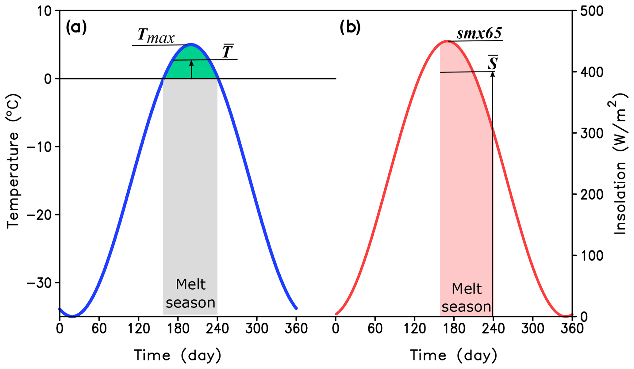
Figure A1 Typical seasonal variations of surface air temperature (a) and insolation (b) at the location of glacial inception.

The parameter δ in Eq. (A9) represents the sensitivity of maximum summer temperature to CO₂ concentration. It can be expressed through other known parameters as δ=p_ar_fc_s, where p_a is the “polar amplification” of maximum summer temperature equal to $\mathrm{\Delta }{T}_{\max }/\mathrm{\Delta }{T}_{\mathrm{g}}$, where ΔT_g is the global air temperature anomaly caused by CO₂ concentration change; r_f is the parameter determining the radiative forcing of CO₂,

$$\begin{array}{}\text{(A11)}& \mathrm{\Delta }{R}_{{\mathrm{CO}}_{\mathrm{2}}}=r_{\mathrm{f}}\ln \left({\displaystyle \frac{{\mathrm{CO}}_{\mathrm{2}}}{{\mathrm{CO}}_{{\mathrm{2}}_{\mathrm{0}}}}}\right);\end{array}$$

and c_s is the specific climate sensitivity (e.g., Rohling et al., 2012), which relates the global temperature change to radiative forcing:

$$\begin{array}{}\text{(A12)}& \mathrm{\Delta }{T}_{\mathrm{g}}=c_{\mathrm{s}}\mathrm{\Delta }R.\end{array}$$

Based on IPCC 2021 (2021) and climate model simulations p_a=1.5, r_f=5.7 W m⁻² and c_s=0.75 °C W⁻¹ m², which is equivalent to an equilibrium climate sensitivity of 3 °C. Thus δ=6.4 °C. To derive a critical relationship between insolation and CO₂ for triggering glacial inception, we make use of the fact that the glacial inception occurs when the total snowmelt minus refreezing during the melt season does not exceed annual snowfall P (in kg m⁻²), which for the considered region is less than 200 kg m⁻²:

$$\begin{array}{}\text{(A13)}& \stackrel{\mathrm{‾}}{M}\mathrm{\Delta }{t}_{\mathrm{M}}={\displaystyle \frac{P}{\mathrm{1}-f_{\mathrm{r}}}},\end{array}$$

where Δt_M is the duration of the melt season and f_r is an average refreezing fraction of snowmelt. Thus, Eq. (A6) can be rewritten as

$$\begin{array}{}\text{(A14)}& \begin{array}{rl}& k_{\mathrm{S}}(\mathrm{1}-{\mathit{\alpha }}_{\mathrm{s}})\mathit{\tau }\cdot \mathrm{smx}\mathrm{65}+k_{\mathrm{T}}(\mathit{\beta }+\mathit{\gamma })\left(\mathit{\delta }\ln {\displaystyle \frac{{\mathrm{CO}}_{\mathrm{2}}}{{\mathrm{CO}}_{{\mathrm{2}}_{\mathrm{0}}}}}+\mathit{\mu }\cdot \mathrm{smx}\mathrm{65}\right)\\ & ={\displaystyle \frac{PL}{(\mathrm{1}-f_{\mathrm{r}})\mathrm{\Delta }{t}_{\mathrm{M}}}}+\mathit{\sigma }{T}_{\mathrm{0}}^{\mathrm{4}}-F\left(\mathrm{0}\right)\\ & -k_{\mathrm{T}}(\mathit{\beta }+\mathit{\gamma })\left(T_{\max }^{*}-\mathit{\mu }\cdot \mathrm{smx}{\mathrm{65}}^{*}\right),\end{array}\end{array}$$

which can be rewritten in the form

$$\begin{array}{}\text{(A15)}& \mathrm{smx}{\mathrm{65}}_{\mathrm{cr}}=A-B\ln {\displaystyle \frac{{\mathrm{CO}}_{\mathrm{2}}}{{\mathrm{CO}}_{{\mathrm{2}}_{\mathrm{0}}}}}.\end{array}$$

This is identical to the relationship proposed in Ganopolski et al. (2016). Here

$$\begin{array}{}\text{(A16)}& \begin{array}{rl}A& =\\ & {\displaystyle \frac{PL(\mathrm{1}-f_{\mathrm{r}}{)}^{-\mathrm{1}}\mathrm{\Delta }{t}_{\mathrm{M}}^{-\mathrm{1}}+\mathit{\sigma }{T}_{\mathrm{0}}^{\mathrm{4}}-F(\mathrm{0})+k_{\mathrm{T}}(\mathit{\beta }+\mathit{\gamma }\left)\right(\mathit{\mu }\cdot \mathrm{smx}{\mathrm{65}}^{*}-T_{\max }^{*})}{k_{\mathrm{S}}(\mathrm{1}-{\mathit{\alpha }}_{\mathrm{s}})\mathit{\tau }+k_{\mathrm{T}}\mathit{\mu }(\mathit{\beta }+\mathit{\gamma })}}\end{array}\end{array}$$

and

$$\begin{array}{}\text{(A17)}& B={\displaystyle \frac{k_{\mathrm{T}}\mathit{\delta }(\mathit{\beta }+\mathit{\gamma })}{\left(k_{\mathrm{S}}\right(\mathrm{1}-{\mathit{\alpha }}_{\mathrm{s}})\mathit{\tau }+k_{\mathrm{T}}\mathit{\mu }(\mathit{\beta }+\mathit{\gamma })}}.\end{array}$$

We will start from determining B, which can be calculated using the following values of model parameters: α_s=0.7, which is a typical albedo of melting snow; τ=0.5 is taken from Robinson et al. (2010), β=4 $\mathrm{W}{\mathrm{m}}^{-\mathrm{2}}\mathrm{°}{\mathrm{C}}^{-\mathrm{1}}$ (derived from the regression of model data for the considered region), γ=15 W m⁻² °C⁻¹ (middle of the range from Braithwaite, 2009) and μ=0.08 W⁻¹ m² °C (from climate model simulations for different orbital parameters). However, since $k_{\mathrm{S}}(\mathrm{1}-{\mathit{\alpha }}_{\mathrm{s}})\mathit{\tau }=\mathrm{0.13}\ll k_{\mathrm{T}}(\mathit{\beta }+\mathit{\gamma })=\mathrm{0.9}$, Eq. (A17) for B can be significantly simplified, and only two parameters are required:

$$\begin{array}{}\text{(A18)}& B={\displaystyle \frac{\mathit{\delta }}{\mathit{\mu }}}\approx \mathrm{80}\mathrm{W}{\mathrm{m}}^{-\mathrm{2}}.\end{array}$$

Equation (A16) for A contains a number of parameters which are not accurately known. However, knowledge of all these parameters is not required. It is only essential that the value of A for different glacial inceptions should remain approximately constant. This requirement is satisfied since only the total snowfall depends on the values of insolation and CO₂ in this formula. However, the contribution of the latent heat term PL(1−f_r)Δt_M to the value of A is only about 10 %–20 %, and, according to climate model simulations, changes in annual precipitation for a wide range of CO₂ concentrations are of the same magnitude. Thus, the total variations of A across the considered range of climate conditions should not exceed a few percent. This allows us to determine A using two paleoclimate constraints, namely that glacial inceptions occurred at the end of MIS19 and 11, while no glacial inception occurred in the recent past (see also Fig. 3b in Ganopolski et al., 2016). These empirical constraints suggest that under the present-day maximum summer insolation of 479 W m⁻², glacial inception can only occur if the CO₂ concentration is around 240 ppm. This gives the following value:

$$\begin{array}{}\text{(A19)}& A=\mathrm{479}+\mathrm{80}\ln {\displaystyle \frac{\mathrm{240}}{\mathrm{280}}}\approx \mathrm{467}\mathrm{W}{\mathrm{m}}^{-\mathrm{2}}.\end{array}$$

Note that the choice of critical CO₂ for present-day insolation of 240 ± 20 ppm results in an uncertainty of A of only ±6 W m⁻². Equation (A15) now can be rewritten as

$$\begin{array}{}\text{(A20)}& \mathrm{smx}{\mathrm{65}}_{\mathrm{cr}}\left[\mathrm{W}{\mathrm{m}}^{-\mathrm{2}}\right]=-\mathrm{80}\cdot \ln {\displaystyle \frac{{\mathrm{CO}}_{\mathrm{2}}\left[\mathrm{ppm}\right]}{\mathrm{280}}}+\mathrm{467},\end{array}$$

which is numerically very similar to Ganopolski et al. (2016) and the results of the present study.

Equation (A18) for B has a clear physical sense: the slope of the critical relationship between insolation and the logarithm of CO₂ concentration is equal to the ratio between local temperature sensitivities to CO₂ (δ) and summer insolation (μ). This value has dimension W m⁻². If one wants to compare the effect of insolation to the effect of radiative forcing of CO₂ in the same units of W m⁻², then it would be $B/r_{\mathrm{f}}=\mathrm{15}$; i.e., 1 W m⁻² of CO₂ forcing is approximately equivalent to 15 W m⁻² of the maximum summer insolation in determining the glacial inception. This number is consistent with the results of earlier studies (Calov and Ganopolski, 2005; Abe-Ouchi et al., 2013).