the Creative Commons Attribution 4.0 License.
the Creative Commons Attribution 4.0 License.
 | 17 May 2024
The role of atmospheric CO2 in controlling sea surface temperature change during the Pliocene
Alan M. Haywood
Julia C. Tindall
Aisling M. Dolan
Daniel J. Hill
Erin L. McClymont
Sze Ling Ho
Heather L. Ford
We present the role of CO2 forcing in controlling Late Pliocene sea surface temperature (SST) change using six models from Phase 2 of the Pliocene Model Intercomparison Project (PlioMIP2) and palaeoclimate proxy data from the PlioVAR working group. At a global scale, SST change in the Late Pliocene relative to the pre-industrial is predominantly driven by CO2 forcing in the low and mid-latitudes and non-CO2 forcing in the high latitudes. We find that CO2 is the dominant driver of SST change at the vast majority of proxy data sites assessed (17 out of 19), but the relative dominance of this forcing varies between all proxy sites, with CO2 forcing accounting for between 27 % and 82 % of the total change seen. The dearth of proxy data sites in the high latitudes means that only two sites assessed here are predominantly forced by non-CO2 forcing (such as changes to ice sheets and orography), both of which are in the North Atlantic Ocean.
We extend the analysis to show the seasonal patterns of SST change and its drivers at a global scale and at a site-specific level for three chosen proxy data sites. We also present a new estimate of Late Pliocene climate sensitivity using site-specific proxy data values. This is the first assessment of site-specific drivers of SST change in the Late Pliocene and highlights the strengths of using palaeoclimate proxy data alongside model outputs to further develop our understanding of the Late Pliocene. We use the best available proxy and model data, but the sample sizes remain limited, and the confidence in our results would be improved with greater data availability.
- Article
(5143 KB) - Full-text XML
-
Supplement
(3435 KB) - BibTeX
- EndNote


The Late Pliocene (∼3.6–2.6 Ma), particularly the mid-Piacenzian Warm Period (mPWP; 3.264–3.025 Ma), is a key focus of palaeoclimate research as one of the best potential “analogues” in terms of climate response for the near-term future (e.g. Budyko, 1982; Zubakov and Borzenkova, 1988; Haywood et al., 2011; Burke et al., 2018; Tierney et al., 2020; Forster et al., 2021). This implies that the Late Pliocene can provide important context for future climate change, particularly given that it is the most recent period of sustained warmth above pre-industrial (PI) levels, has an atmospheric CO2 concentration elevated above PI levels, and has a similar continental configuration to modern day. Furthermore, estimates of equilibrium climate sensitivity (ECS) from past warm periods like the Late Pliocene can act as useful constraints to current estimates of ECS and consequently inform our understanding of the response of the climate system to CO2 forcing.
Over the past 35 years, there has been a concerted effort to collate and synthesise disparate geological information from the Late Pliocene to build a progressively more complete spatial picture of the patterns of change. In particular, in the last decade, the reconstruction efforts of the modelling and data–model communities have adopted a “time slice” approach and focused on a specific interglacial period within the Late Pliocene. Selected as the target for Phase 2 of the Pliocene Model Intercomparison Project (PlioMIP2; Haywood et al., 2016a) and the upcoming Phase 3 (PlioMIP3; Haywood et al., 2024), Marine Isotope Stage (MIS) KM5c is a warm interval with orbital forcing very similar to the modern and characterised by a negative benthic oxygen isotope excursion (0.21 ‰–0.23 ‰) centred on 3.205 Ma (Lisiecki and Raymo, 2005; Haywood et al., 2013). KM5c also has an atmospheric CO2 concentration similar to the modern, with a central estimate of 371 ppm (de la Vega et al., 2020).
In addition to these synthesis efforts, additional proxy data from new sites, and at higher temporal resolution, mean that we are beginning to better understand the temporal variability in the Late Pliocene, but understanding the cause of the changes we see in proxy records for a specific site remains difficult. Here, we integrate a novel modelling method with the best available Late Pliocene geological sea surface temperature (SST) data to gain insight into the causes of sea surface temperature change during the Late Pliocene.
1.1 Synthesis of recent geological data
The U.S. Geological Survey Pliocene Research Interpretation and Synoptic Mapping (PRISM) project has been instrumental in documenting geological data for the Pliocene for over 3 decades. PRISM reconstructions have been used in both phases of PlioMIP: PlioMIP1, assessing the mPWP, used the PRISM3D reconstruction (Dowsett et al., 2010), while PlioMIP2, assessing the KM5c time slice, used the PRISM4 reconstruction (Dowsett et al., 2016).
Alongside the PRISM project, the Past Global Changes (PAGES) PlioVAR working group has also compiled geological data with a remit of assessing Pliocene climate variability on glacial–interglacial timescales, including the mPWP and the following period of intensified Northern Hemisphere glaciation (McClymont et al., 2017, 2020a, 2023a). The PlioVAR working group developed robust stratigraphic constraints that allowed a detailed view of ocean temperatures during KM5c; full details on the age models used are presented in McClymont et al. (2020a).
Two proxy reconstructions of SST are included in the PlioVAR KM5c synthesis, namely from alkenones, using the index, and from planktonic foraminifera MgCa proxies (McClymont et al., 2020a; see also Sect. 2.3). Mid-Piacenzian SSTs have previously also been reconstructed (e.g. O'Brien et al., 2014; Petrick et al., 2015; Rommerskirchen et al., 2011) using the TEX86 proxy (Schouten et al., 2002), but these data were not included in the PlioVAR KM5c synthesis as they could not be confidently assigned to the KM5c interval (McClymont et al., 2020a). Results from the and MgCa proxy data were used in tandem and also compared to assess the impact of the choice of proxy for SST reconstruction.
The combined and MgCa proxy data produced a global annual mean SST anomaly of +2.3 °C for KM5c relative to the PI, with the largest anomalies in the mid- and high latitudes and a reduction in the meridional SST gradient of 2.6 °C. This global mean SST warming derived from the two proxies is equal to the warming shown in the PlioMIP2 ensemble mean, with 10 models indicating less warming than this, and 6 models indicating more warming (McClymont et al., 2020a).
PlioVAR has also examined the climate following KM5c and the onset and intensification of Northern Hemisphere glaciation (McClymont et al., 2023a). An updated planktonic foraminifera MgCa reconstruction was created as part of this analysis, covering the KM5c interval. Assessing Pliocene climate variability on a longer timescale reinforces the idea that targeting a specific interglacial allows for the best data–model comparison efforts due to the minimisation of orbital-scale variability (McClymont et al., 2020a, 2023a; Haywood et al., 2020).
1.2 Using climate models to aid interpretation of geological data
Despite the long history of geological data synthesis, understanding the cause of a given climate signal remains challenging. As climate models have developed, their ability to be used synergistically alongside geological proxy data has increased, and there is now a strong precedent for using models to support the interpretation of proxy data (e.g. Salzmann et al., 2008, 2013; Tindall et al., 2017).
There are multiple ways in which this synergistic model–proxy data relationship can be explored. On a basic level, we can compare proxy data to model data to test how well signals of change are reconstructed in a given time period; proxy data and models agreeing on the sign and amplitude of change gives us confidence in both methods and suggest an ability to use models to explore the drivers and processes behind signals seen in proxy data. Conversely, disagreement between proxy data and models can lead to a decrease in confidence and questions around the cause of different signals (Tindall et al., 2022; see also Haywood et al., 2016b; McClymont et al., 2020a). Such disagreements reveal the shortcomings and limitations of either the proxies and/or the climate models and outline avenues to further improve them.
Climate models are also capable of simulating some original proxy signals (e.g. the isotopic signal incorporated into plant wax δD; see Knapp et al., 2022) rather than the variable calculated from the proxy, which includes additional sources of potential uncertainty in its derivation. In turn, models can help our understanding of what might be controlling the proxy signal in a given time and space. For example, Tindall et al. (2017) use an isotope-enabled version of the HadCM3 model to directly simulate pseudo-coral and pseudo-foraminifera data in the Pacific to explore the expression of El Niño in the Pliocene. Using isotope-enabled models in this way, it is possible to see regions where the isotopic expression of the El Niño–Southern Oscillation (ENSO) is pronounced (e.g. the central Pacific; Tindall et al., 2017), which allows us to assess whether the proxy data signal at specific sites is driven by ENSO or another form of variability.
Palaeoclimate proxy data and modelling outputs have also been used synergistically to constrain estimates of climate sensitivity, particularly for the Late Pliocene (e.g. Hargreaves and Annan, 2016, and references therein; Haywood et al., 2020) and the Last Glacial Maximum (e.g. Renoult et al., 2020). Hargreaves and Annan (2016) present an estimate of ECS of 1.9–3.7 °C for the mPWP using PlioMIP1 model output and proxy data from PRISM3 (Dowsett et al., 2009). Haywood et al. (2020) extend and adapt this analysis for the PlioMIP2 model outputs and generate a site-specific estimate of ECS using the mPWP SST reconstruction of Foley and Dowsett (2019).
Here we present another example of using climate model outputs and geological proxy data synergistically to build a clearer picture of Late Pliocene environmental change by exploring the dominant cause of SST change at specific proxy data sites. We apply the FCO2 method of Burton et al. (2023; detailed in Sect. 2.1) using outputs from PlioMIP2 to explore the local forcings at individual proxy sites with reference to CO2 forcing and palaeogeographic boundary condition changes. We then discuss the implications of these results, including what the model output may indicate at a seasonal scale that the proxy data cannot resolve (Sect. 4.1), and present a new estimate of Late Pliocene climate sensitivity (Sect. 4.2).
2.1 FCO2 method
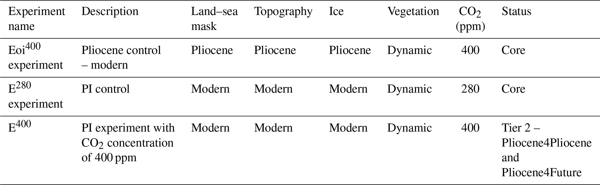
The FCO2 method was first presented in Burton et al. (2023) and shows the proportion of the total Pliocene minus PI climate change that is due to CO2 forcing. The method uses three experiments from PlioMIP2: Eoi400, E280, and E400 (Table 1). At the time of compiling this study, six modelling groups had completed the E400 experiment for SST, and these six models are used as a subset of the PlioMIP2 ensemble (see Sect. 2.2).
Table 1Names and descriptions of the three PlioMIP2 experiments used in the FCO2 method (Burton et al., 2023).
FCO2 is calculated by
where E400–E280 represents the change in climate caused by the change in CO2 concentration from 280 to 400 ppm alone, and Eoi400–E280 represents the change in climate as a result of implementing the full Pliocene boundary conditions. Although this paper focuses on SST change, the FCO2 method can be applied to any climate parameter so long as the necessary model experiments (Table 1) have been run.
The FCO2 calculation typically produces a result between 0 and 1, where 1 represents a change wholly dominated by CO2 forcing, and 0 represents the opposite case where change is wholly dominated by non-CO2 forcing. In keeping with the PlioMIP2 experimental design, non-CO2 forcing is defined as changes to ice sheets and orography, the latter of which also includes changes to prescribed vegetation, bathymetry, land–sea mask, soils, and lakes (Haywood et al., 2016a).
FCO2 values above 1 and below 0 can occur in rare instances (see Burton et al., 2023). If the effect of CO2 forcing is in the opposite direction to the overall climate signal (i.e. E400–E280>0 but Eoi400–E280<0 or E400–E280<0 but Eoi400–E280>0), then FCO2 will be below 0. If the effect of CO2 forcing is greater than the overall climate signal (i.e. E400–E280 > Eoi400–E280>0 or E400–E280 < Eoi400–E280<0), then FCO2 will be above 1. Such values are mostly commonly seen where the Eoi400–E280 anomaly is small, and the usefulness of the FCO2 method is limited in these cases where there is little climate signal to explain.
The FCO2 method is only suited to quantifying the proportion of the total change that is attributable to CO2 forcing or non-CO2 forcing. The method alone cannot expand on the underlying physical mechanisms or processes, though it is possible to make suggestions based on, for example, knowledge of the oceanographic setting at a given proxy site. In order to comment further on the non-CO2 forcings, it would be necessary to complete further forcing factorisation model experiments, which is beyond the scope of this paper but is a suggested target for future modelling work looking towards PlioMIP3 (see Haywood et al., 2024).
In this paper, as in Burton et al. (2023), uncertainty in the FCO2 analysis is considered in terms of whether there is consistent agreement between the individual models on whether CO2 forcing (FCO2>0.5) or non-CO2 forcing (FCO2<0.5) is the most important driver of change. FCO2 is deemed to be uncertain in regions where three or fewer of the six models agree on the dominant forcing.
2.2 Participating models and model boundary conditions
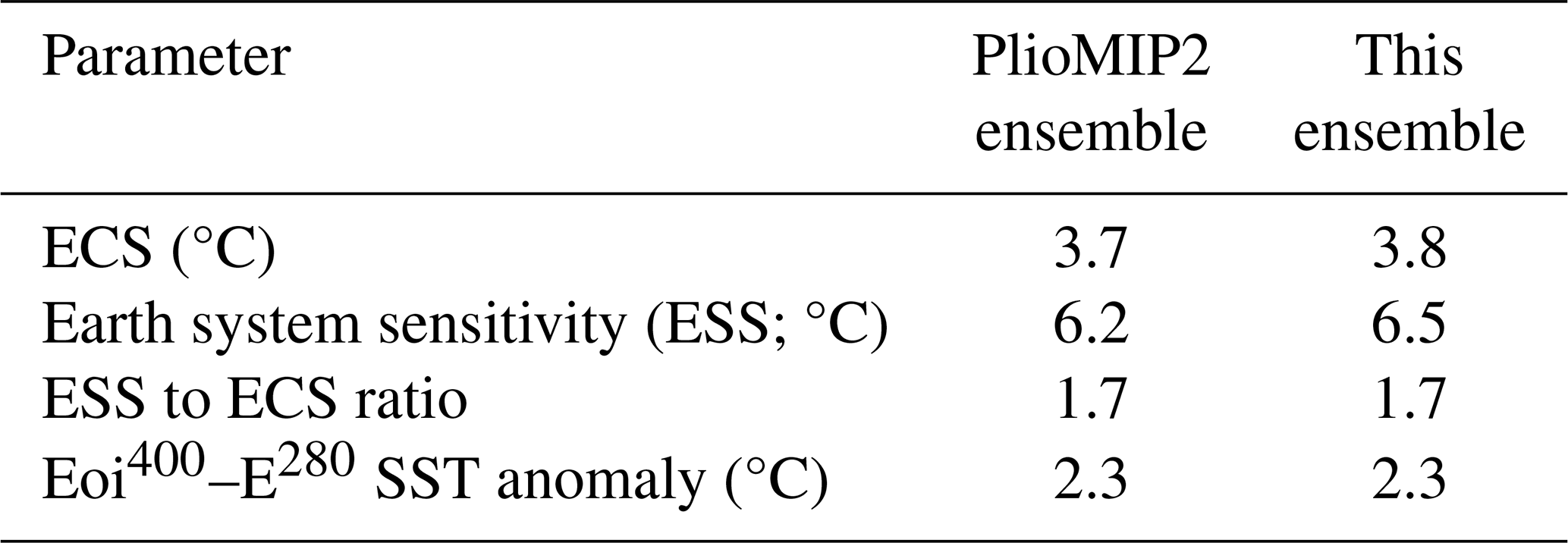
For a model to be included in this study, it had to meet the criteria of completing the Eoi400, E280, and E400 experiments for SST, with outputs spun up to equilibrium. Of the 17 models included in PlioMIP2, 6 met these criteria: CCSM4-UoT, CESM2, COSMOS, HadCM3, MIROC4m, and NorESM1-F. The models vary in age and resolution; summary details are shown in Burton et al. (2023), and full details for the PlioMIP2 ensemble are shown in Haywood et al. (2020). This subset of models is representative of the whole PlioMIP2 ensemble (Table 2). Standardised Pliocene boundary conditions are used in all models in PlioMIP2 – including the six models here – which are derived from the U.S. Geological Survey PRISM4 reconstruction (Dowsett et al., 2016) and implemented as described in Haywood et al. (2016a).
Table 2A comparison of climate parameters between the PlioMIP2 ensemble and the subgroup of PlioMIP2 models used in this study (adapted from Burton et al., 2023; the adaptation reflects the exclusion of the IPSLCM5A2 climate model from this SST-focused ensemble due to limited model data availability).
The boundary conditions include spatially complete gridded datasets at 1°×1° of latitude–longitude for land–sea distribution, topography and bathymetry, vegetation, soil, lakes, and land ice cover, and all models here used the “enhanced” version, meaning that they include reconstructed changes to the land–sea mask and ocean bathymetry (Haywood et al., 2020). The Pliocene palaeogeography is similar to the modern, except for the closure of the Bering Strait and Canadian Arctic Archipelago, increased land area in the Maritime Continent, and a West Antarctic seaway (Haywood et al., 2016a; Dowsett et al., 2016). The PRISM4 reconstruction also includes dynamic topography and glacial isostatic adjustment to better represent local sea level (Dowsett et al., 2016). The atmospheric concentration of CO2 is set to 400 ppm in the PlioMIP2 boundary conditions, with concentrations for all other trace gases set as identical to those in the PI control experiment (E280) for each individual model group (Haywood et al., 2016a).
The ice configuration in the PRISM4 reconstruction is based upon the results from the Pliocene Ice Sheet Modelling Intercomparison Project (PLISMIP; Dolan et al., 2015). The Greenland ice sheet is confined to high elevations in the eastern Greenland mountains, covering an area of around 25 % of the modern ice sheet (Dolan et al., 2015; Koenig et al., 2015). The ice coverage over Antarctica is still a source of debate (see Levy et al., 2022), but the PRISM3 reconstruction (Dowsett et al., 2010) is supported and so retained in the PRISM4 reconstruction (Dowsett et al., 2016). This configuration sees a reduction in the ice margins in the Wilkes and Aurora basins in eastern Antarctica, while western Antarctica is largely ice-free.
2.3 Proxy SST data
The temporal focus of this paper is MIS KM5c (3.205±0.01 Ma), the time slice used in PlioMIP2. Details on KM5c, the age models used, and the data assigned to KM5c are presented in McClymont et al. (2020a). We adopt a multi-proxy approach using data from the PlioVAR project (McClymont et al., 2020b, 2023b). Two SST proxies are assessed: the alkenone-derived index (Prahl and Wakeham, 1987) and foraminifera calcite MgCa (Delaney et al., 1985). Both proxies have multiple calibrations to modern SST, and the impact of calibration choice on SST data is discussed in McClymont et al. (2020a). As for the PlioVAR analyses (McClymont et al., 2020a, 2023a), SST data were generated using the same calibration for all and MgCa measurements to minimise the impact of calibration choice on differences between sites.
As in McClymont et al. (2020a), anomalies relative to the PI are calculated using the ERSSTv5 dataset. We focus on the BAYSPLINE calibration for alkenone-derived SST data (Tierney and Tingley, 2018) and an updated PlioVAR calibration for MgCa SST data (McClymont et al., 2023a). Hereafter, “ data” will refer to the BAYSPLINE dataset presented in McClymont et al. (2020a, b), and “MgCa data” will refer to the MgCa dataset presented in McClymont et al. (2023a, b); “PlioVAR data” will refer to both of these datasets in combination. The choice of calibration does not significantly impact the FCO2 on SST results (see Sect. S1 in the Supplement).
Seven sites presented in McClymont et al. (2020a) are not included here as they fall on land in the model Pliocene land–sea mask, meaning that a FCO2 on SST value cannot be generated. Four of these sites are also in the Benguela upwelling region, the driving processes for which are not well captured by current climate models. Though FCO2 on surface air temperature (SAT) is shown to be comparable to FCO2 on SST outside of the high latitudes in Burton et al. (2023), the decision was made to exclude these sites as a site-specific comparison could not be made, and taking the nearest ocean grid point may not accurately represent the oceanographic setting of the proxy site.
The sites considered here have also been analysed for the PRISM3 time interval (3.264–3.025 Ma; Dowsett et al., 2010). Data for the PRISM3 interval are only considered in the temporal variability analysis (Sect. 3.2) and represent the mean of the entire period rather than a warm peak average so are well suited to assessing temporal variability. No data from the PRISM3 interval are available for site U1337, so this site is also excluded from the analysis for completeness. All data in all other sections are solely for KM5c.
In total, 21 proxy sites are considered. Of these, 19 proxy sites have data available for KM5c, 15 of which have data and 6 of which have MgCa data (sites U1313 and ODP1143 have data from both proxy types). Site ODP999 has only MgCa data available for KM5c but MgCa data and data for the PRISM3 interval. The remaining two sites (DSDP610 and U1307) have data available for the PRISM3 interval only (with no data available for KM5c) and are included in Sect. 3.2 only.
3.1 FCO2 on sea surface temperature
The location of the proxy sites with reference to the multi-model mean (MMM) Eoi400–E280 SST anomaly and FCO2 on SST are shown in Fig. 1. The MMM global mean Eoi400–E280 SST anomaly is 2.3 °C with a global mean FCO2 value of 0.56, indicating that 56 % of the warming (1.29 °C) is predominantly driven by CO2 forcing. Warming is amplified at high latitudes and is greatest in the Labrador Sea and North Atlantic region (for full analysis of meridional and zonal trends in the PlioMIP2 ensemble, see Haywood et al., 2020). Full interpretation of FCO2 on SST is presented in Burton et al. (2023).
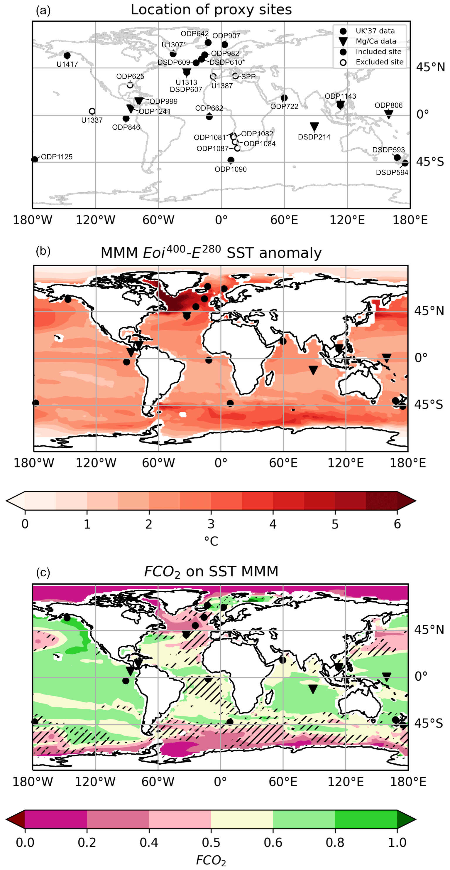
Figure 1Location of PlioVAR proxy data sites (a). sites are denoted by a circle, and MgCa sites are denoted by a triangle. Filled symbols indicate that the site is used in this paper; open symbols indicate that the site is not used either because no model SST values are available at the site and/or because analysis had not been conducted for the PRISM3 interval and KM5c. Sites marked with an asterisk (*) only have data available for the PRISM3 interval (no data are available for KM5c) and are only considered in the temporal variability analysis (Sect. 3.2). Sites included in this paper are shown again in panel (b) with the MMM Eoi400–E280 SST anomaly and in panel (c) with the FCO2 on SST MMM. The MMM comprises CCSM4-UoT, CESM2, COSMOS, HadCM3, MIROC4m, and NorESM1-F. Hatching in panel (c) denotes regions of uncertainty in FCO2, defined as regions where three or fewer models agreed on the dominant forcing (i.e. whether FCO2<0.5 or FCO2>0.5).
CO2 forcing is dominant in the low and mid-latitudes, and non-CO2 forcing becomes more dominant in the high latitudes, indicating that meridional gradients may have a mixture of drivers (e.g. the tropical Atlantic, with a FCO2 between 0.5–0.8, is predominantly driven by CO2 forcing, whereas the North Atlantic, with a FCO2 between 0.2–0.5, is predominantly driven by non-CO2 forcing). Given the spatial pattern of FCO2 on SST (Fig. 1c), it is clear that the lack of proxy data sites available in the high latitudes limits the identification of sites where SST is predominantly driven by non-CO2 forcing. Aside from the North Atlantic, regions with low FCO2 (FCO2<0.5) – the Arctic Ocean, parts of the northern Pacific Ocean, and the Southern Ocean – have a relative dearth of proxy data sites available for the KM5c time slice.
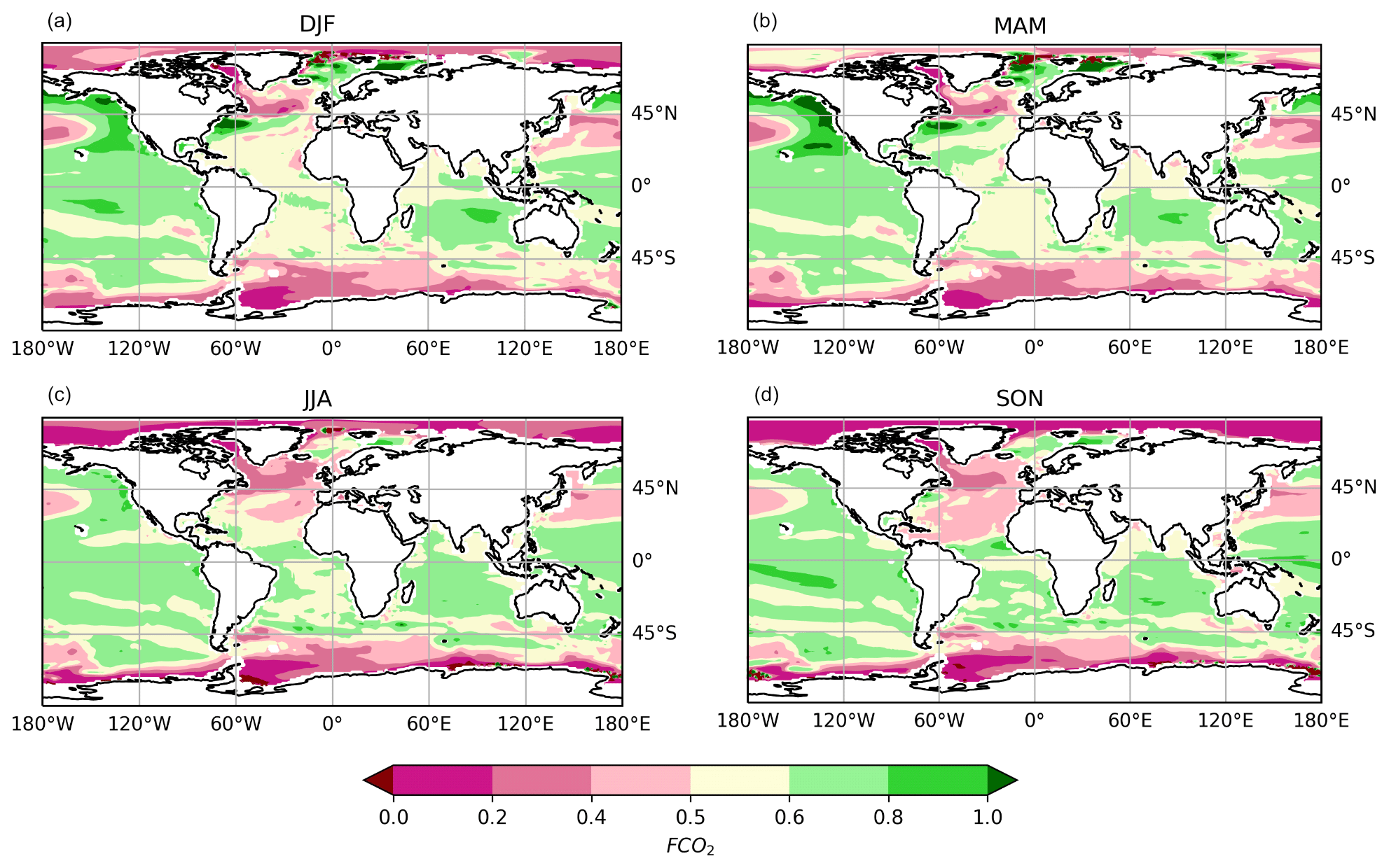
Figure 2Seasonal variation in FCO2 on SST MMM shown for the months of December, January, and February (DJF) (a); March, April, and May (MAM) (b); June, July, and August (JJA) (c); and September, October, and November (SON) (d). The MMM comprises CCSM4-UoT, CESM2, COSMOS, HadCM3, MIROC4m, and NorESM1-F.
The broad-scale pattern of CO2 forcing being dominant at low and mid-latitudes and non-CO2 forcing being dominant at high latitudes persists throughout the year and does not change significantly between the seasons (Fig. 2). While the spatial patterns of FCO2 on SST may not significantly change, the relative strength of the dominant forcing can be seen to differ.
In some regions, such as the North Atlantic, it is possible to see seasonal differences in both the spatial pattern of the dominant forcing and its relative influence. Non-CO2 forcing is dominant in the northern North Atlantic basin in the months of December, January, and February (DJF; Fig. 2a) and March, April, and May (MAM; Fig. 2b), the influence of which extends southward in June, July, and August (JJA; Fig. 2c) to a maximum extent in September, October, and November (SON; Fig. 2d). The region of low FCO2 that extends throughout the year has relatively mixed forcing (FCO2 0.4–0.5), while a smaller region of more dominant non-CO2 forcing (FCO2 0.2–0.4) remains relatively constrained between 45 and 55° N, and 60 to 20° W.
The FCO2 method provides spatial detail on the drivers of climate change and associated gradients, but it alone cannot provide further information on the specific mechanisms and processes behind the change(s) seen. The FCO2 method allows us to comment on the collective role of non-CO2 forcing (representing both ice sheets and orography combined), but it does not allow us to comment on, for example, the role of ice sheets alone or the separate components encapsulated by “orography” in the PlioMIP2 experiments (orography, bathymetry, land–sea mask, lakes, soils, and prescribed vegetation; Haywood et al., 2016a). To do this, more model experiments would be needed which further factorise the effects of ice vs. orography (see Haywood et al., 2016a).
3.1.1 FCO2 on sea surface temperature at individual proxy data sites
The KM5c-PI SST anomaly at the majority of proxy data sites analysed (17 out of 19) is predominantly driven by CO2 forcing (Table 3). Of these sites, 1 (U1417) was highly dominated by CO2 forcing (FCO2 0.8–1.0), 10 were dominated by CO2 forcing (FCO2 0.6–0.8), and the remaining 6 sites experienced more mixed forcing (FCO2 0.5–0.6).
Table 3FCO2 classes and their interpretation (adapted from Burton et al., 2023) with associated KM5c proxy data sites. Sites marked with an asterisk (*) are in regions of uncertainty in FCO2, defined where three or fewer models agreed on the dominant forcing (i.e. whether FCO2<0.5 or FCO2>0.5).
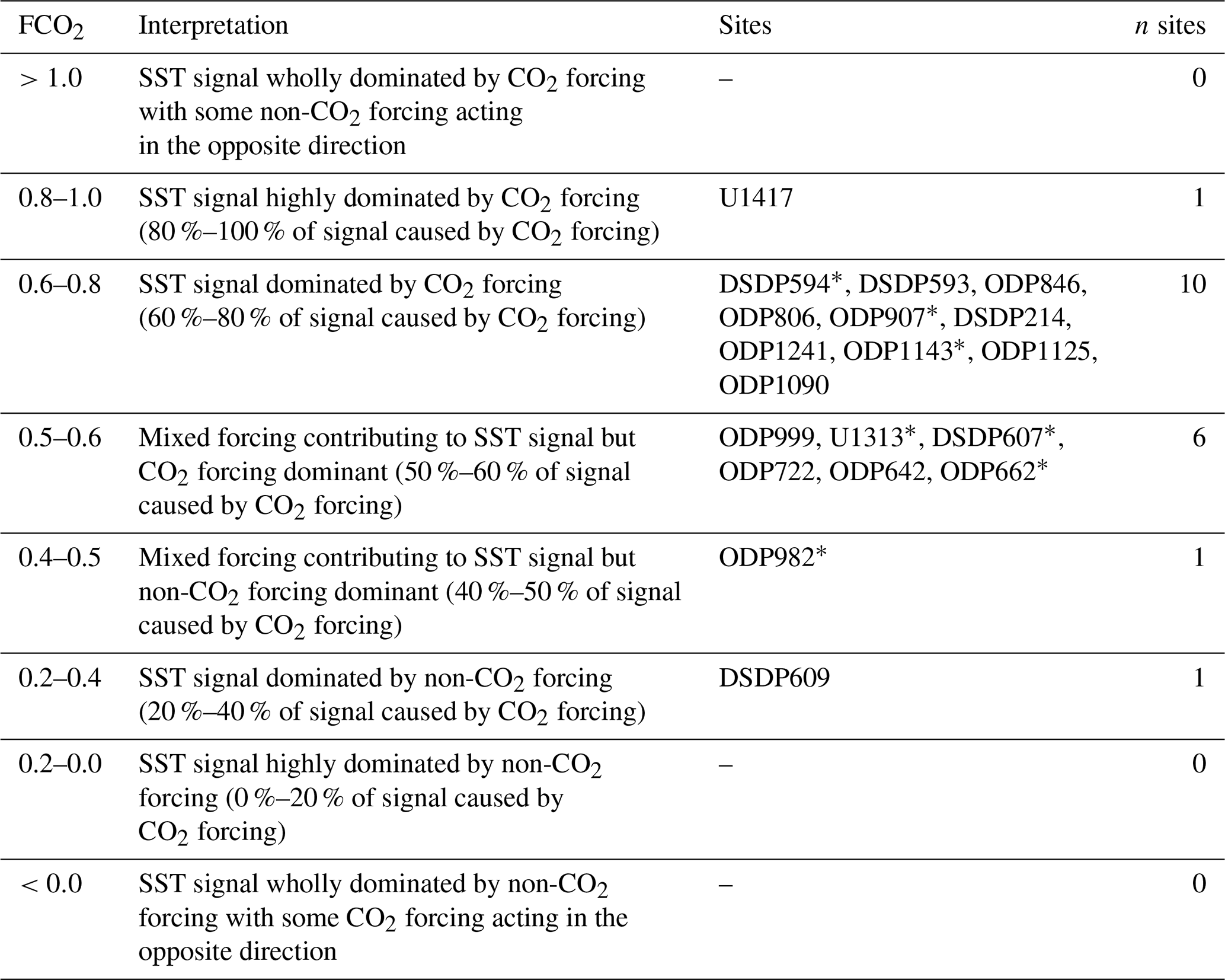
The Southern Hemisphere mid-latitude sites (DSDP593, DSDP594, ODP1125, and ODP1090) are all dominated by CO2 forcing (FCO2 0.6–0.8), as are the sites in the tropical Pacific (ODP806, ODP846, and ODP1241). Only sites ODP982 and DSDP609 are predominantly influenced by non-CO2 forcing, and both are situated in the North Atlantic. Furthermore, the majority of sites with FCO2 between 0.5–0.6 are also interconnected via the low-, mid-, and high-latitude North Atlantic.
Each site was assessed for uncertainty in FCO2 between the six models (i.e. whether FCO2<0.5 or FCO2>0.5 in three or fewer of the models; hatching in Fig. 1c). Proxy sites are generally found where the models show agreement on the dominant forcing; however, there are seven sites that do not. Of these seven sites, two have both and MgCa data available (U1313 and ODP1143), and five have only data available (ODP907, ODP982, DSDP607, ODP662, and DSDP594).
Of the 19 sites analysed, 11 had good data–model agreement between the reconstructed and simulated SST response (hereafter referred to as the “data–model agreement”). Here we consider data–model agreement in terms of the difference between the MMM Eoi400–E280 SST anomaly and the KM5c proxy data–ERSSTv5 PI anomaly; sites that fall within ±2 °C are considered to have good data–model agreement, and sites that fall within ±0.5 °C are considered to have very good data–model agreement (Table 4).
Table 4Site-specific FCO2 and data–model agreement at sites with data for KM5c.
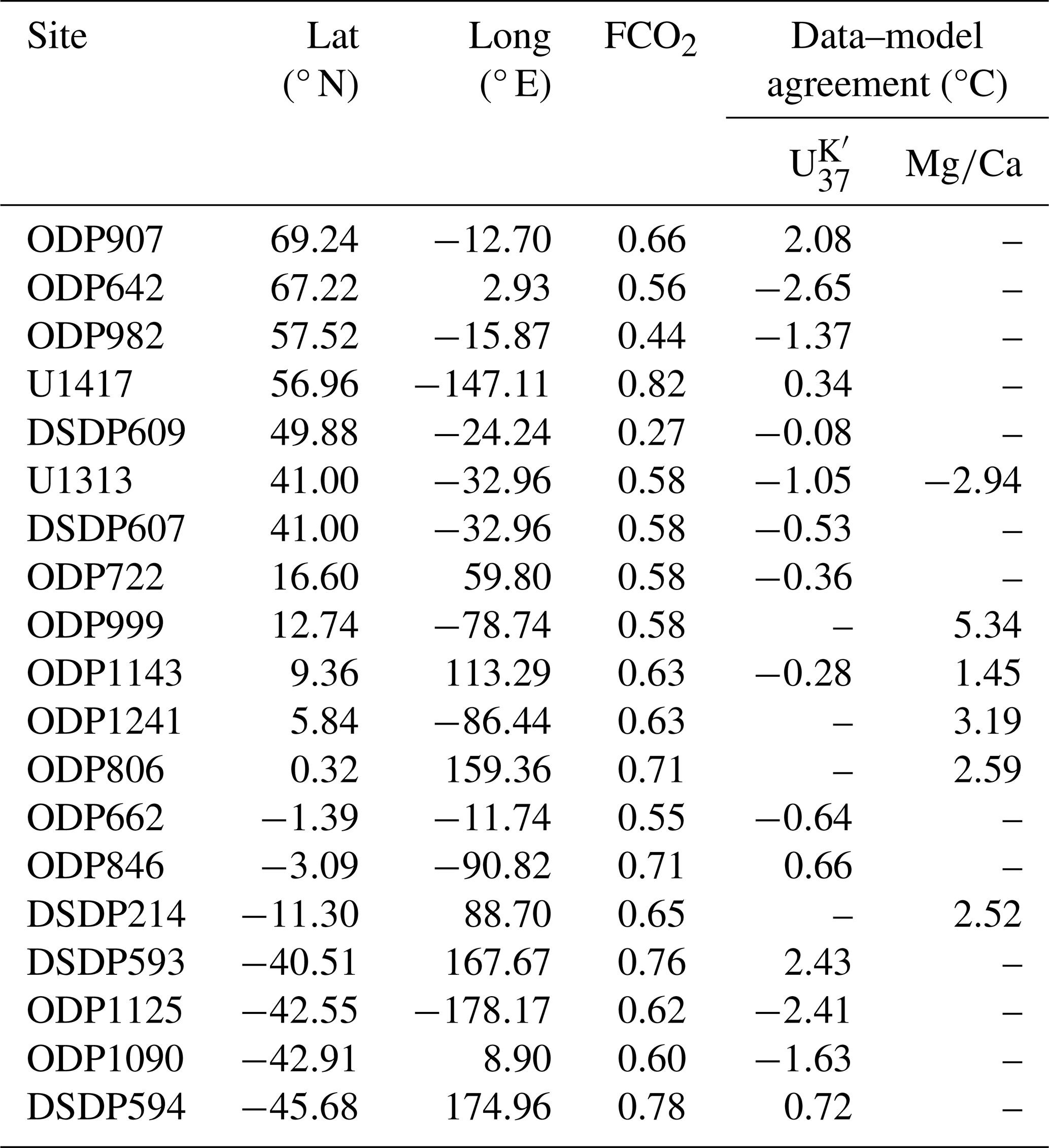
Seven sites have good data–model agreement (light blue symbols in Fig. 3), and four have very good agreement (dark blue symbols in Fig. 3). The spatial distribution of these sites is representative of the total number of sites assessed, including the clustering of sites in the North Atlantic. In constraining the focus of the rest of our FCO2 analysis to sites with good data–model agreement (pie charts in Fig. 3), we should get the clearest and most accurate view of Late Pliocene SST change and its drivers.
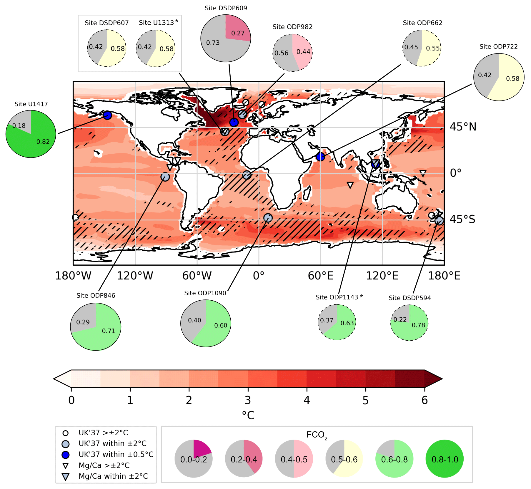
Figure 3MMM Eoi400–E280 SST anomaly represented by the background red shading. The MMM comprises CCSM4-UoT, CESM2, COSMOS, HadCM3, MIROC4m, and NorESM1-F. Hatching represents uncertainty in FCO2, where three or fewer of the six models agree on the dominant forcing (i.e. whether FCO2<0.5 or FCO2>0.5). The shape of the overlying symbols denotes the type of proxy data at each site (circle = ; triangle = MgCa), and the colour of the symbol represents the level of data–model agreement (darker = stronger agreement). All proxy data are for KM5c. The site-specific FCO2 on SST MMM is represented with a pie chart at each proxy site where there is good data–model agreement (i.e. the MMM Eoi400–E280 SST anomaly is within at least ±2 °C of the proxy data SST anomaly). The proportion of the pie chart that is coloured denotes the proportion of total change attributable to CO2 forcing (i.e. the FCO2), which is also represented by the colour. Smaller pie charts with a dashed outline denote sites where there is uncertainty between models on the dominant forcing (i.e. where there is hatching on the main plot). Sites U1313 and ODP1143, marked by an asterisk (*), have both and MgCa data available; both the data and the MgCa data are within at least ±2 °C for site ODP1143, but only the data are within ±2 °C for site U1313.
Sites ODP1143 and U1313 have both and MgCa data available. At site ODP1143, there is very good data–model agreement (within ±0.5 °C) when using the data and good data–model agreement (within ±2 °C) when using the MgCa data. There is good data–model agreement (within ±2 °C) when using the data at site U1313, but the MgCa data have relatively poor data–model agreement ( °C). The remaining sites with good data–model agreement are represented by data only.
The range in FCO2 on SST values indicates how the relative dominance of CO2 forcing varies between all of the proxy sites, with CO2 forcing driving between 27 % and 82 % of the total change seen. CO2 is the dominant forcing accounting for the difference in SST between KM5c and the PI at 9 of the 11 sites with good data–model agreement (Fig. 3). Site U1417 is highly dominated by CO2 forcing with a MMM FCO2 on SST of 0.82; sites ODP1090, ODP846, ODP1143, and DSDP594 are dominated by CO2 forcing (FCO2 0.6–0.8); and sites ODP662, DSDP607, U1313, and ODP722 have more mixed forcing, though CO2 remains dominant (FCO2 0.5–0.6). In contrast, sites DSDP609 and ODP982 in the North Atlantic are predominantly driven by non-CO2 forcing (FCO2 0.27 and 0.44, respectively); these are the only two proxy sites included in this study where this is the case.
It is worth noting that six of these sites (ODP662, DSDP607, U1313, ODP982, ODP1143, and DSDP594) show uncertainty in the FCO2 on SST between models (smaller pie charts with dashed outlines in Fig. 3; see Table S2 and Fig. S2 for individual model values). This means that three or fewer of the six models agree on the dominant forcing (i.e. whether FCO2>0.5 or FCO2<0.5), and hence, conclusions should be drawn with caution given the uncertainty between the models.
3.1.2 Proxy data–model agreement
All KM5c proxy data sites were explored to assess whether the FCO2 method could provide insight into the reason for the (lack of) data–model agreement. For example, if the data–model agreement is better where FCO2 is high, then the non-CO2 forcing in the models may be inaccurate. Given the differences in oceanographic settings of the proxy data sites included, we hypothesise that any relationship would be site-dependent.
To assess whether there was a relationship between FCO2 on SST and data–model agreement, the FCO2 on SST and Eoi400–E280 anomaly for each of the six models were also individually assessed. Regardless of whether the data–model agreement was very good, good, or poor, there was no consistent or significant relationship between FCO2 and data–model agreement (Fig. 4). Values of FCO2 above 1 and below 0 had the potential to skew any relationships and were seen at multiple sites and in multiple models.
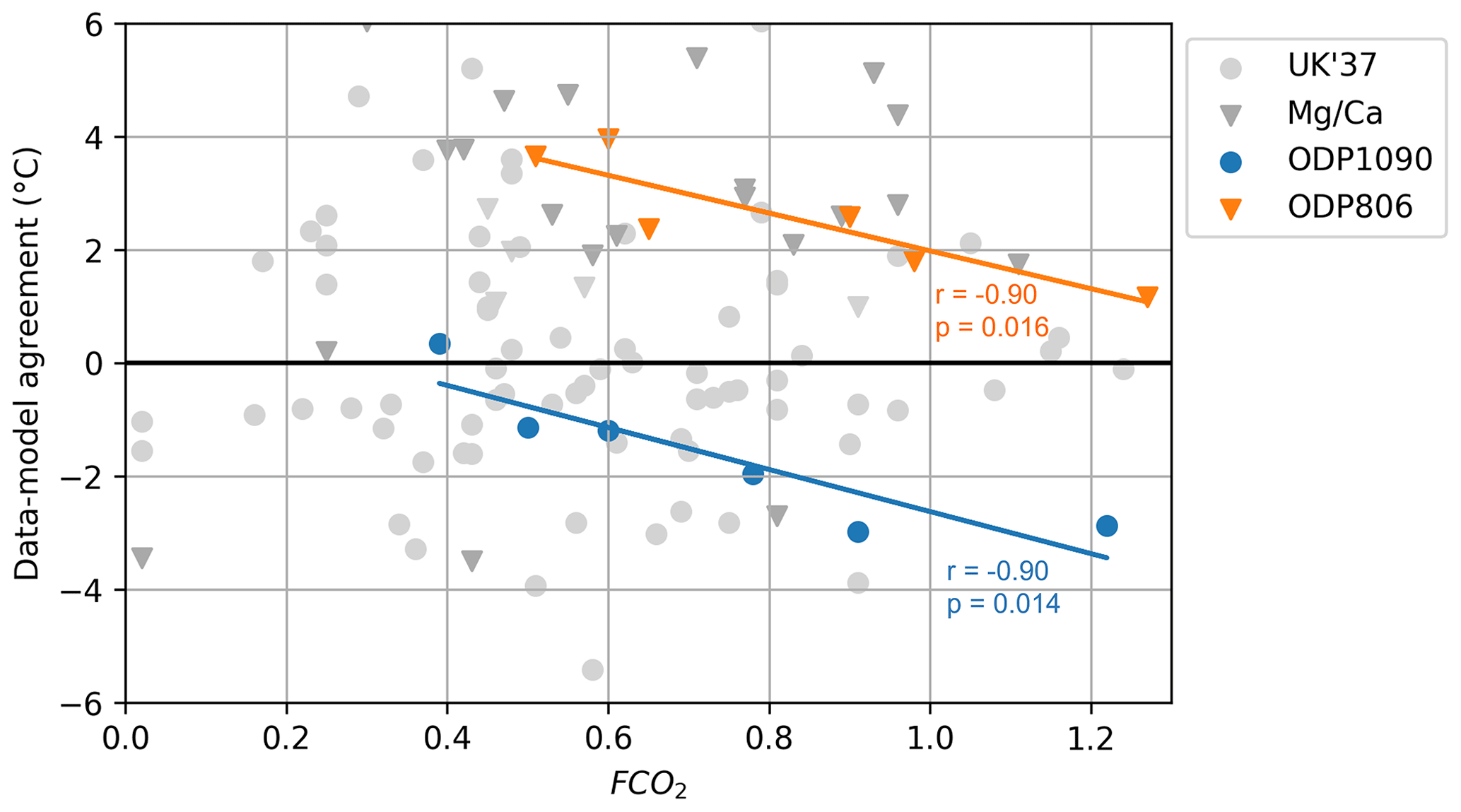
Figure 4The relationship between individual model FCO2 and the data–model agreement for all KM5c proxy sites considered here. data are represented by circles, and MgCa data are represented by triangles. Only the two sites with a significant relationship are coloured: site ODP1090 in blue circles and MgCa site ODP806 in orange triangles. Note that the FCO2 scale extends to 1.3 to include values from all six models. Some data points with extreme FCO2 values lie outside of the FCO2 range included in this figure, but the axes' limits allow the significant relationships at sites ODP1090 and ODP806 to be demonstrated clearly.
Only two sites showed a statistically significant relationship: ODP1090 (blue circles in Fig. 4) and ODP806 (orange triangles in Fig. 4). There is a negative relationship between FCO2 and data–model agreement at site ODP1090 (; p=0.014; blue in Fig. 4). Data–model agreement varies from 0.35 °C (CESM2) to −2.98 °C (NorESM1-F) with a MMM of −1.63 °C, and FCO2 on SST varies from 0.39 (CESM2) to 1.22 (COSMOS) with a MMM of 0.60. If COSMOS is excluded due to the FCO2 value above 1, the relationship further strengthens (; p=0.0023). CESM2, the only model with a FCO2 value smaller than 0.5 (indicating that non-CO2 forcing is dominant), has the best data–model agreement. This relationship – of models with higher FCO2 having worse data–model agreement – may suggest that the influence of CO2 forcing is overestimated in some of the models and/or that the models underestimate the influence of non-CO2 forcings at site ODP1090.
There is also a negative relationship between FCO2 and data–model agreement at site ODP806 (; p=0.016; orange in Fig. 4). Data–model agreement varies from 1.17 °C (NorESM1-F) to 3.96 °C (COSMOS) with a MMM of 2.59 °C, and FCO2 on SST varies from 0.51 (CESM2) to 1.27 (NorESM1-F) with a MMM of 0.71. NorESM1-F has the best data–model agreement and the highest FCO2 value; even if it is excluded because of the FCO2 value above 1, the relationship remains strong and statistically significant (; p=0.048). This relationship – of models with higher FCO2 having better data–model agreement – may suggest that non-CO2 forcing has too large an impact at site ODP806 in models with lower FCO2. It is worth noting, however, that site ODP806 is the only site assessed for which all six models agree that CO2 is the dominant forcing; i.e. where all six models have a FCO2 on SST > 0.5 (CESM2 has the lowest FCO2 on SST value at 0.51).
Though the subset of models considered here is shown to be representative of the whole PlioMIP2 ensemble (Table 2), our confidence in the relationship between FCO2 and data–model agreement seen at sites ODP1090 and ODP806 is linked to the overall sample size and inherent uncertainty in both the models and proxy data. The hypothesis that the relationship would be site-dependent is found to be true, though many of the relationships seen were not statistically significant, so our confidence in this conclusion is limited. It also appears that the relationship may be dependent on the proxy type: the cool bias in the MgCa SST data discussed in McClymont et al. (2020a) is visible in Fig. 4 (MgCa data represented by the grey triangles), with the majority of data–model comparison values above 0 °C. MgCa data also appear to have poorer data–model agreement than the data, though commenting on the reasons for this is beyond the scope of this paper.
3.2 Temporal variability
We hypothesise that sites with a lower FCO2 (i.e. sites where non-CO2 forcing was more dominant) could experience greater temporal variability in forcing and therefore in temperature response to forcing feedbacks. This is because, on orbital timescales, there could be changes in the ice sheet and vegetation components of the non-CO2 forcing and/or changes in sea ice. Changes in ice sheets, vegetation, and sea ice are more likely to affect the regions that are more influenced by non-CO2 forcing (i.e. regions with lower FCO2). These are mainly the higher latitudes, but more distant regions can also be affected by the movement of the thermal Equator that occurs with polar ice changes and other such feedbacks.
By assessing SST proxy data from the PRISM3 interval (3.264–3.025 Ma), it is possible to comment on the temporal variability seen in the SST proxy data results and how that compares and relates to the FCO2 analysis. This was investigated using the standard deviation as an approximation for temporal variability (Fig. 5).
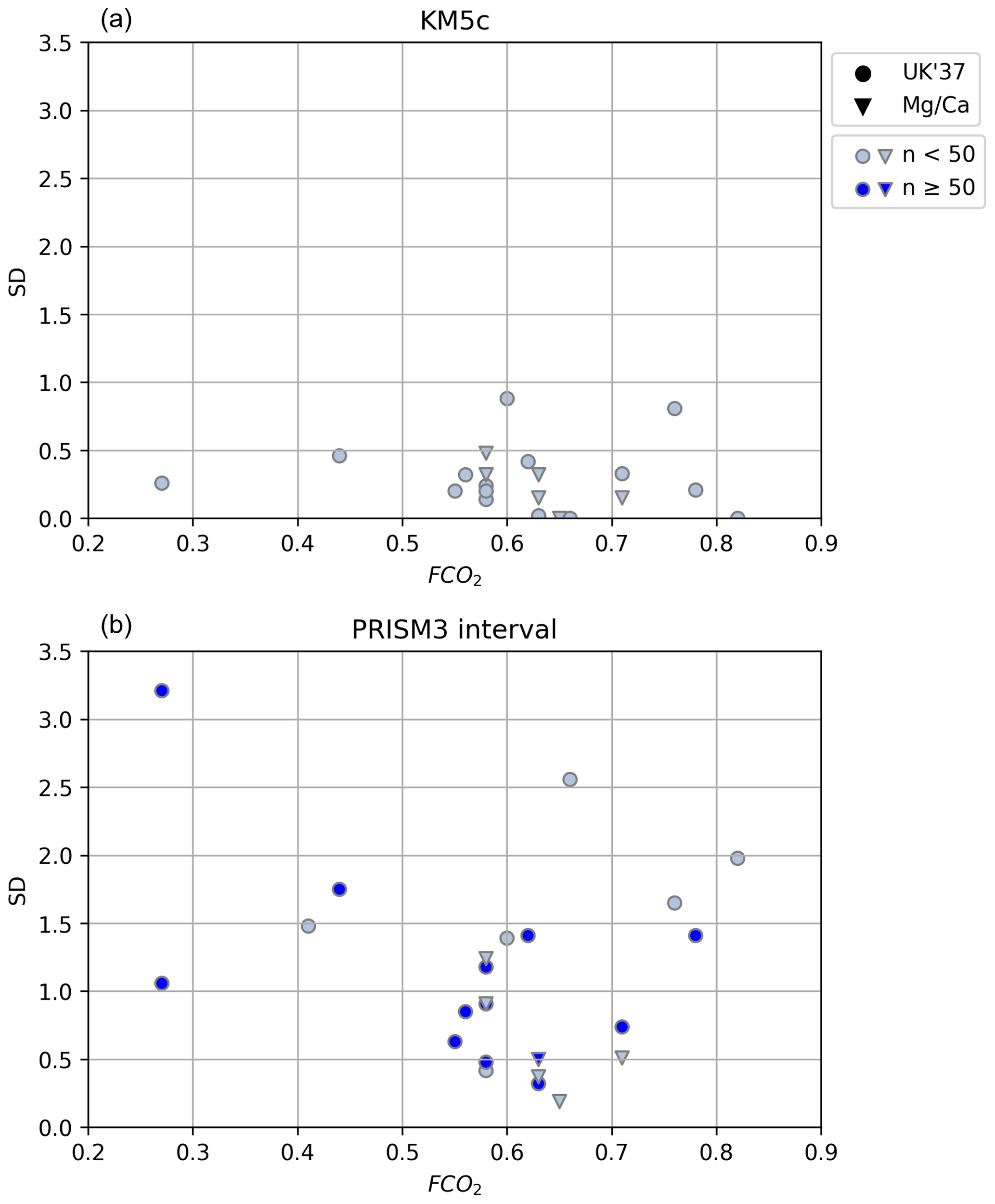
Figure 5FCO2 on SST MMM compared to standard deviation (SD) of SST proxy data for KM5c (a) and the PRISM3 interval (b). data are represented by circles, and MgCa data are represented by triangles. Sites are grouped into two classes according to the number of data points available: sites with fewer than 50 data points are shown in light blue, and sites with greater than or equal to 50 data points are shown in dark blue.
Table 5Sampling densities at proxy sites. Note that two sites (U1313 and ODP1143) have and MgCa data available for both KM5c and the PRISM3 interval, and a further site (ODP999) has only MgCa data available for KM5c but both MgCa and data available for the PRISM3 interval.
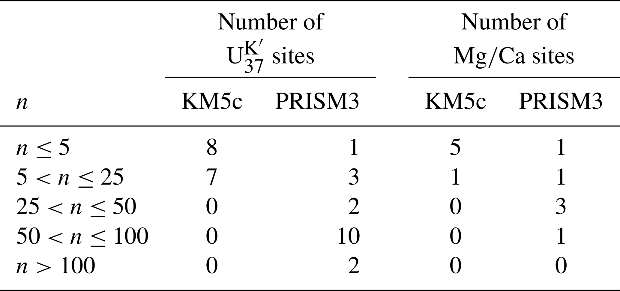
The relationship between FCO2 and standard deviation is highly sensitive to the sample size, and it is clear that an increase in both the number of sites and the number of data points at each site is needed to explore this relationship further. If one focuses on KM5c, the maximum sampling density at a given site is 10 ( at sites ODP1125 and ODP722). It was therefore necessary to consider the PRISM3 interval to capture a greater range in standard deviation and hence temporal variability estimates. Furthermore, because KM5c was chosen as a target for analysis in part due to its low variability (Haywood et al., 2013; McClymont et al., 2020a), one would only expect significant variability to be seen in the PRISM3 interval. In total, 21 proxy data sites have data available for the PRISM3 interval, with sampling densities ranging between 4 (MgCa at site DSDP214) and 125 ( at site ODP722).
In total – accounting for both and MgCa data for KM5c and the PRISM3 interval – 15 sites have a sample size less than or equal to 5, and 12 sites have a sample size between 5 and 25 (Table 5; see Table S3 for site names). If sites with a sample size greater than or equal to 50 only (dark blue symbols in Fig. 5) are considered (by default, therefore only looking at the PRISM3 interval), the hypothesised relationship – high FCO2 sites experience lower temporal variability – is seen (; p=0.070). Though the hypothesised relationship is seen, our confidence is limited due to the relatively low data availability, highlighting the need for more data availability at both existing and new proxy sites. No relationship is seen for sites with a sample size smaller than 50, regardless of whether data from KM5c are included (r=0.10; p=0.59) or excluded (r=0.18; p=0.32).
More work is needed to further explore this relationship. In particular, future modelling efforts could calculate FCO2 from other time slices within the PRISM3 interval, as the FCO2 results here only represent the influence of forcing on the climate during KM5c. These results are presented here with an awareness of this limitation and nonetheless still represent the best exploration possible, given the model and proxy data currently available.
4.1 FCO2 and seasonality
We show that CO2 forcing is the main driver of SST change for KM5c relative to the PI at most of the proxy sites assessed (Sect. 3.1.1) and that FCO2 on SST varies seasonally at a global scale (Sect. 3.1). To further explore the potential for seasonal reconstructions of FCO2 to inform the interpretation of specific SST proxy records, it is necessary to consider FCO2 at a local (site-specific) level. We present seasonality in both FCO2 on SST MMM and the MMM Eoi400–E280 SST anomaly for three individual proxy sites, which provides a possible framework for the discussion regarding the climate signal recorded in the proxy data. Though the seasonality in simulated SST is model-dependent, the models are consistent enough to begin to suggest trends that may be useful when interpreting the proxy data.
Three sites are selected as examples (Fig. 6), though it is possible to conduct this analysis for any of the sites included in this paper. Site DSDP609, in the North Atlantic, has the lowest annual mean FCO2 on SST (0.27) in the collection of sites presented. Site U1417, in the Gulf of Alaska, has the highest annual mean FCO2 on SST (0.82). Site ODP1090 is one of the most southern sites presented and has an annual mean FCO2 on SST of 0.60. The proxy data are taken to reflect the annual mean, and proxy values of each of these sites are presented with two uncertainty estimates, ±1 and ±2 °C (orange shading in Fig. 6). Calculating site- and proxy–data-type-specific uncertainties is beyond the scope of this paper, so these uncertainty estimates represent a simple thought experiment that approximate plausible uncertainty values purely to provide the necessary context (i.e. magnitude of seasonality seen in FCO2 vs. limitations of reproducing the magnitude of temperature changes from the proxy record).
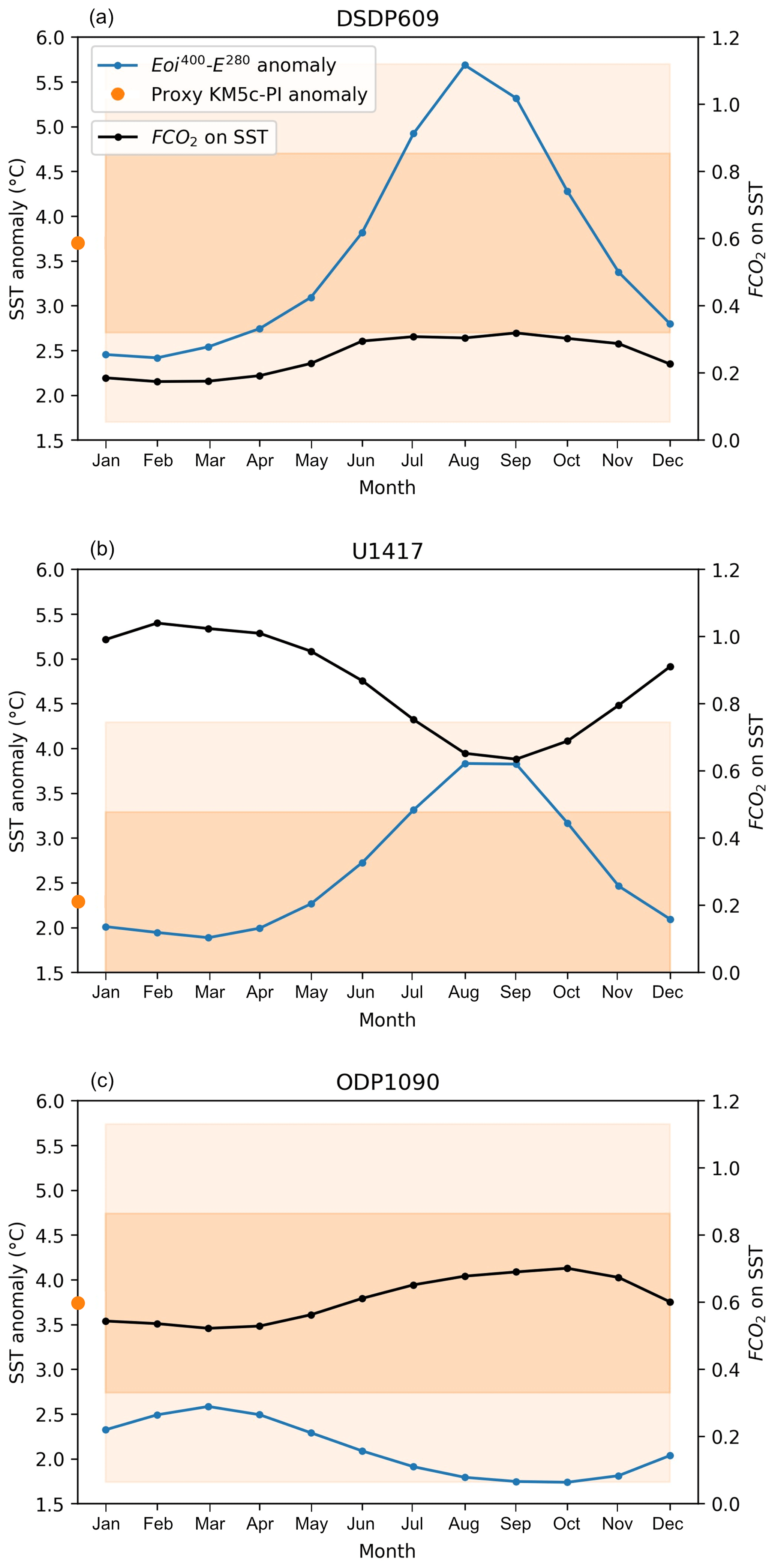
Figure 6Monthly MMM Eoi400–E280 SST anomaly (blue line) and FCO2 on SST (black line) at sites DSDP609 (a), U1417 (b), and ODP1090 (c). The proxy data KM5c-PI anomaly value is shown by the orange circle on the y axis, with plausible uncertainty estimates shown by orange shading (darker orange denoting ±1 °C; lighter orange denoting ±2 °C). Note that the scale for FCO2 on SST extends to 1.2 as some monthly values exceed 1.0 for site U1417.
There is a large seasonal variation in the Eoi400–E280 anomaly at site DSDP609 (Fig. 6a), with the smallest anomaly (2.45 °C) in January and maximum anomaly (5.69 °C) in August. The proxy data anomaly of 3.70 °C is well matched to the MMM annual mean Eoi400–E280 anomaly of 3.62 °C, and all of the model seasonality is captured within ±2 °C of the proxy data value (blue line within orange shading in Fig. 6a). Though there is large seasonal variation in the Eoi400–E280 anomaly, the total range in FCO2 on SST is relatively small. FCO2 increases between January (0.18) and September (0.32), suggesting that CO2 forcing has a proportionally greater role in the warming in this period. Despite this, site DSDP609 is always either highly dominated (FCO2 0.0–0.2) or dominated (FCO2 0.2–0.4) by non-CO2 forcing.
The magnitude of the seasonal variation in the Eoi400–E280 anomaly is smaller at site U1417 than at site DSDP609, but there is greater variation in FCO2 on SST (from 0.63 (September) to 1.04 (February); Fig. 6b). The smallest Eoi400–E280 anomalies are seen at the start of the year and culminate in the greatest warming in the late summer and early autumn months. The proxy data anomaly of 2.29 °C is smaller than the mean annual MMM anomaly of 2.63 °C, which could suggest that the models overestimate the magnitude of the summer/autumn peak in warming and/or that the peak is not fully represented in the proxy data, but the data–model agreement is very good, and all model seasonality is within ±2 °C of the proxy data (blue line within orange shading in Fig. 6b). FCO2 clearly decreases throughout MAM and JJA as the Eoi400–E280 anomaly increases, indicating that the greatest warming is attributable to changes in non-CO2 forcing. Interestingly, FCO2 on SST is above 1 for February (1.04), March (1.02), and April (1.01), which, given the overall warming signal, indicates that there is a small role of non-CO2 forcing in cooling the SST. However, the overall signal of change is dominated by CO2 forcing throughout the year, and the lowest FCO2 on SST is 0.55 in May (indicating mixed forcing with CO2 forcing dominant).
Compared to DSDP609 and U1417 in the Northern Hemisphere mid-latitudes, site ODP1090 shows little seasonal variation in the Eoi400–E280 anomaly (Fig. 6c). The greatest warming is seen in the summer (DJF) and autumn (MAM) seasons, with a total annual variation from 1.74 °C in October to 2.58 °C in March. The proxy data anomaly of 3.74 °C is over a degree warmer than the warmest month in the model data (March; 2.58 °C), which may indicate either that the models do not accurately represent the degree of warming and/or that the proxies overestimate the warming. The months with least warming in the models (August–November) are at the low end of the plausible proxy data uncertainties used (blue line within light orange shading in Fig. 6c). The FCO2 remains fairly consistent throughout the year – ranging from 0.52 (March) to 0.70 (October) – and CO2 is always the dominant forcing. Months with the lowest FCO2 are also the months with the greatest Eoi400–E280 anomaly, indicating that this warming can be attributed to non-CO2 forcing (e.g. changes to positions of the front systems associated with the Antarctic Circumpolar Current or Antarctic Ice Sheet, though the FCO2 method alone cannot detail the exact non-CO2 forcing components).
These results highlight the usefulness of the FCO2 method in terms of understanding the drivers of seasonal trends in SST change at the individual site level. Though it is beyond the scope of this paper, comparing the model-derived SST anomaly and FCO2 with different proxy systems and/or different calibration methods used within a particular proxy system may shed light on and resolve proxy data biases, as well as data–model discrepancies. Furthermore, it may be interesting to complete a seasonal analysis for sites with different oceanographic settings; the three sites presented here represent a range in FCO2 but may not be representative of the range in seasonality seen between all proxy sites.
4.2 Constraints on site-specific climate sensitivity estimates
There is a discernible relationship between ECS and the ensemble-simulated Pliocene SAT anomaly within the PlioMIP2 ensemble (Haywood et al., 2020). Quantifying the influence of CO2 forcing at individual proxy data sites using the FCO2 method means that it is now possible to better determine which sites may be best placed to inform estimates of ECS.
The modelled tropical oceans are particularly strongly related to modelled ECS, indicating that it is possible to constrain estimates of ECS using Pliocene SST data from the tropics. Haywood et al. (2020) used the Foley and Dowsett (2019) SST reconstruction (hereafter “FD19”) in this way. They adapted the methodology of Hargreaves and Annan (2016), whereby
where α and C are constants, and ε represents all errors in the regression equation. This methodology was adapted to account for the more sparsely distributed proxy data in PlioMIP2 compared to PlioMIP1 (due to the change in target from the PRISM3 time slab (3.264–3.025 Ma) to the KM5c time slice (3.205 Ma ± 0.01 Ma)) and instead relies on point-based observations and local regressions between Eoi400–E280 SST and modelled ECS.
The adapted methodology applies Eq. (1) with ΔSST from individual data sites and α and C are location-dependent, meaning that sites northward of 30° N and southward of 30° S can also be considered. This produces a different estimate of ECS for each proxy site, though this does not imply that ECS is different for each location (Haywood et al., 2020). Data are presented for sites which meet two conditions: (1) that the relationship between the site-specific Eoi400–E280 SST anomaly and a model's ECS was significant at the 95 % confidence interval and (2) that at least one of the models in the PlioMIP2 ensemble was within ±1 °C of the proxy data (Haywood et al., 2020). If a proxy site fell on land in the Pliocene land–sea mask in the models, the nearest ocean grid point value was taken.
Here we repeat the Haywood et al. (2020) methodology using the PlioVAR data used throughout this paper and the full suite of models in the PlioMIP2 ensemble (see Haywood et al., 2020, for details of the ensemble). We assess the PlioVAR data ECS estimates in the context of FCO2 on SST (Fig. 7a) and compare these results to the original ECS estimates generated from FD19 presented in Haywood et al. (2020) (Fig. 7b).
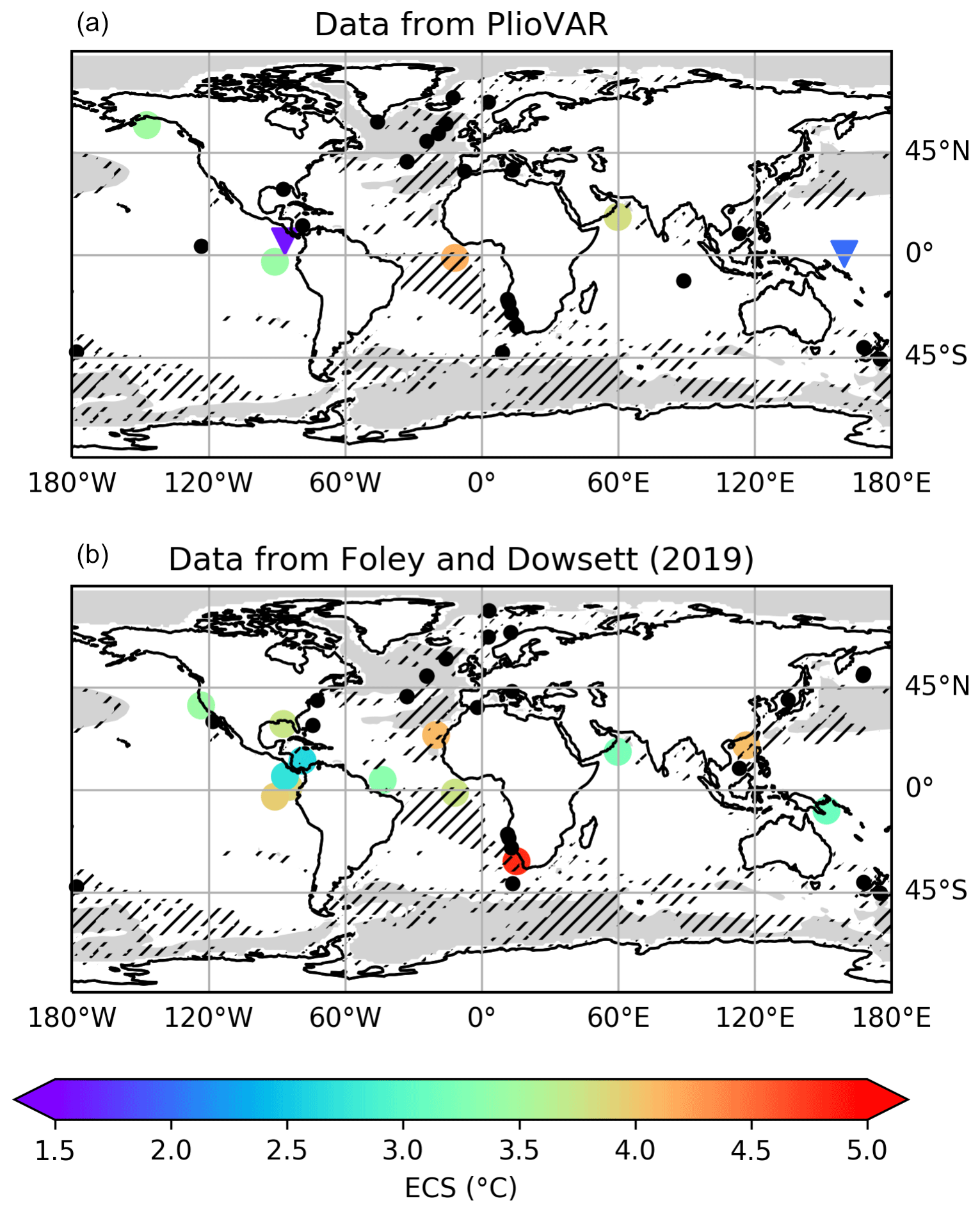
Figure 7KM5c proxy–data-informed ECS estimates. Estimates are calculated using the PlioVAR data used throughout this paper (a) and using FD19 as presented in Haywood et al. (2020) (b). The triangles in panel (a) represent MgCa sites, and circles in panels (a) and (b) represent sites. Coloured symbols denote sites for which an ECS estimate is calculated. The smaller black circles represent sites that did not meet the conditions and were excluded. FCO2 on SST is shown by the background shading; areas in white are predominantly driven by CO2 (FCO2>0.5), and areas in light grey are predominantly driven by non-CO2 forcing (FCO2<0.5). Hatching represents where three or fewer models agree on the dominant forcing (i.e. whether FCO2<0.5 or FCO2>0.5).
Different proxy sites are represented in the results, depending on the dataset chosen, given that the proxy data had to be within ±1 °C of the Eoi400–E280 anomaly of at least one model to be included (i.e. within ±1 °C of the model with the smallest or largest Pliocene minus PI (Eoi400–E280) anomaly). It is important to note that this methodology compares the proxy data to the Eoi400–E280 anomalies for all 17 of the models in the PlioMIP2 ensemble rather than the subset of 6 models used in the remainder of this paper; hence, some sites are included in the climate sensitivity analysis that are not included elsewhere to maximise the number of sites available.
In total, 13 sites are represented using FD19 (Fig. 7b), compared to 6 sites using the PlioVAR data (Fig. 7a). This reduced number partly reflects the additional age constraints applied to the PlioVAR data (see McClymont et al., 2020a). Four sites are represented in both datasets: ODP1241, ODP662, ODP846, and ODP722. Five FD19 sites (ODP625, ODP1018, ODP1087, ODP1115, and ODP1146) met the criteria, but the Pliocene land–sea mask in the models meant that FCO2 on SST was not available; as Burton et al. (2023) show that FCO2 on SAT is comparable to FCO2 on SST outside of the high latitudes, the FCO2 on SAT was taken at these sites as the closest approximation for the climate sensitivity analysis only.
All FD19 data are , using the Müller et al. (1998) calibration, and of the six PlioVAR data sites, four have data (BAYSPLINE calibration) and two have MgCa data. Though the datasets use different calibrations, the difference in reconstructed temperatures is small (see the Supplement of McClymont et al., 2020a). The two MgCa sites do not meet the exact conditions used by Haywood et al. (2020) but are included to begin to explore the applicability of this method to other proxy types; rather than being within ±1 °C of one of the models, the SST proxy data were 1.12 and 1.20 °C cooler than the MMM Eoi400–E280 SST anomaly at sites ODP806 and ODP1241, respectively.
Individual site ECS estimates are shown in Table 6. The original range in estimates presented in Haywood et al. (2020) using FD19 is 2.63 to 4.80 °C. The range broadens to 1.59 to 4.15 °C when using the PlioVAR data, but this is skewed by the two MgCa sites with ECS estimates of 1.99 and 1.59 °C at sites ODP806 and ODP1241, respectively. Both of these ranges are broader but generally align with the likely range of ECS presented in the Sixth Assessment Report of the Intergovernmental Panel on Climate Change (IPCC) of 2.5 to 4.0 °C (Arias et al., 2021). If only the PlioVAR data are considered here (i.e. only those data that meet the original condition of being within ±1 °C of one of the models; Haywood et al., 2020), the range in ECS estimates is constrained to 3.44 to 4.15 °C, which is one of the best constrained estimates of Pliocene ECS to date.
Table 6Proxy sites and their ECS estimates using FD19 and/or the PlioVAR data used in this paper. a Sites are on land in the model Pliocene land–sea mask. b Sites have MgCa data.
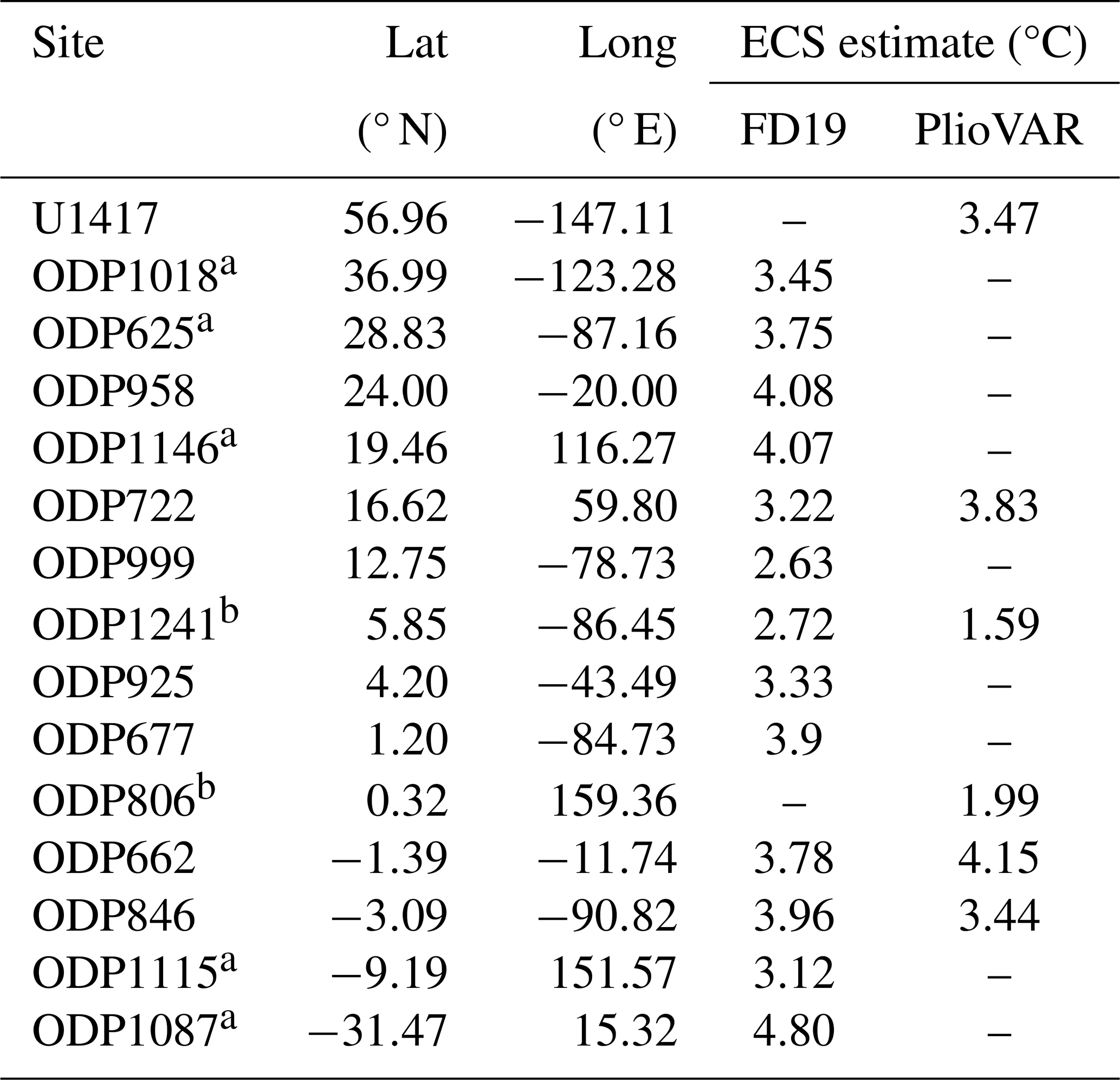
Regardless of the estimate of ECS itself, all of the sites selected using the adapted methodology are in regions where CO2 is the dominant forcing (i.e. where FCO2>0.5; ocean regions in white in Fig. 7). Site ODP662 (present in both the PlioVAR dataset and FD19) has the lowest FCO2 on SST at 0.55, while sites U1417 and ODP846 have the highest FCO2 on SST in the PlioVAR dataset and FD19, respectively, with values of 0.82 and 0.71. Uncertainty in FCO2 on SST (hatching in Fig. 7) is only seen at site ODP662; the remaining sites selected using the adapted methodology show consistent agreement on the dominant forcing of site-specific SST change in at least four of the models.
Sites excluded for not meeting the conditions (small black circles in Fig. 7) are generally found in regions of low FCO2 (FCO2<0.5; grey shading in Fig. 7) and/or in regions of uncertainty in FCO2 (hatching in Fig. 7). Site DSDP214 in the Indian Ocean is an example of an exception to this general rule, but despite the FCO2 on SST being 0.65 (indicating that CO2 forcing is dominant), it is likely to also be influenced by gateway changes (e.g. Karas et al., 2009, 2011). We find that the MgCa data at site DSDP214 do not provide good data–model agreement (2.52 °C; Table 4), and MgCa data sites also appear to generate notably different ECS estimates than sites.
In this way, the FCO2 method could potentially support the selection of sites using the Haywood et al. (2020) methodology for constraining estimates of ECS. At present there are not enough data available to explore whether the proxy-informed estimate of ECS is related to FCO2, but given that there is no significant relationship between ECS and FCO2 on SST in the models used here (see Burton et al., 2023), the potential for finding such a relationship may be unlikely.
We have assessed the role of CO2 forcing in SST change in the Pliocene using the recently introduced FCO2 method (Burton et al., 2023) and the current best available proxy data (McClymont et al., 2020a, 2023a). We focused on SST change due to the relative wealth of KM5c-age proxy data, but a similar exploratory approach could also be adopted for other proxies that provide a quantitative measure of a climate variable, for example, for SAT or precipitation.
Using the climate models and proxy data in tandem, we have explored the forcings behind the SST change more than has previously been possible. We show that the majority of proxy sites are predominantly forced by CO2, and those sites that are not are only found in the North Atlantic. Though a full analysis of zonal and meridional gradients is beyond the scope of this paper, our results also suggest that certain gradients may have multiple contributing drivers and that these drivers may differ by ocean basin and/or by season. We have also presented site-specific seasonal analysis using model data which provides a potential way to gain further insight into how changes in seasonality could be reflected in the reconstructed annual mean temperature change. Both of these components have allowed us to highlight potential reasons for data–model agreement (or lack thereof). A well-constrained, proxy-informed estimate of Pliocene ECS is also presented. Using the latest PlioVAR data, ECS is estimated to be within the range of 1.59 to 4.73 °C and constrained to 3.44 C to 4.73 °C if only data are considered (as in the original methodology presented in Haywood et al., 2020), in line with the estimate presented in the IPCC Sixth Assessment Report.
It is recommended that future work builds on the foundation presented here; the conclusions drawn would be strengthened if more data were available, both from more proxy data sites and from more models running the necessary experiments to apply the FCO2 method. This would set both the palaeoclimate modelling and proxy data communities on track to better understand the climate of the Pliocene and to improve data–model comparison efforts.
The model data required to produce the FCO2 results in this paper are available in the Supplement. The proxy data from McClymont et al. (2020a) are available at https://doi.org/10.1594/PANGAEA.911847 (McClymont et al., 2020b). The proxy data from McClymont et al. (2023a) are available at https://doi.org/10.1594/PANGAEA.956158 (McClymont et al., 2023b). The proxy data from Foley and Dowsett (2019) are available at https://doi.org/10.5066/P9YP3DTV.
The supplement related to this article is available online at: https://doi.org/10.5194/cp-20-1177-2024-supplement.
LEB led the study, analysed the data, and contributed to the writing of the paper. AMH, JCT, AMD, and DJH helped to prepare the paper with contributions from all co-authors. ELM, SLH, and HLF supported the use and integration of marine proxy sea surface temperature data into the paper and contributed to the description of the data as outlined within the paper.
At least one of the (co-)authors is a member of the editorial board of Climate of the Past. The peer-review process was guided by an independent editor, and the authors also have no other competing interests to declare.
Publisher's note: Copernicus Publications remains neutral with regard to jurisdictional claims made in the text, published maps, institutional affiliations, or any other geographical representation in this paper. While Copernicus Publications makes every effort to include appropriate place names, the final responsibility lies with the authors.
For the purpose of open access, the author has applied a Creative Commons Attribution (CC BY) license to any Author Accepted Manuscript version arising. Lauren E. Burton acknowledges that this work was supported by the Leeds–York–Hull Natural Environment Research Council (NERC) Doctoral Training Partnership (DTP) Panorama (grant no. NE/S007458/1). Heather L. Ford acknowledges the Natural Environment Research Council (grant no. NE/N015045/1). The collation and analysis of the PlioVAR data are an outcome of the working group Pliocene Climate Variability over glacial–interglacial timescales, as sponsored by Past Global Change (PAGES). We acknowledge PAGES for their financial support to workshops and discussions and thank all of the PlioVAR members who created, synthesised, reviewed, and analysed the proxy data to generate the PlioVAR data. This research used samples and/or data provided by the International Ocean Discovery Program (IODP), Ocean Drilling Program (ODP), and Deep Sea Drilling Project (DSDP). We acknowledge the PlioMIP2 participants whose data have been used in the support of this study.
This research has been supported by the Natural Environment Research Council (grant no. NE/S007458/1).
This paper was edited by Christo Buizert and reviewed by two anonymous referees.
Arias, P. A., Bellouin, N., Coppola, E., Jones, R. G., Krinner, G., Marotzke, J., Naik, V., Palmer, M. D., Plattner, G.-K., Rogelj, J., Rojas, M., Sillmann, J., Storelvmo, T., Thorne, P. W., Trewin, B., Achuta Rao, K., Adhikary, B., Allan, R. P., Armour, K., Bala, G., Barimalala, R., Berger, S., Canadell, J. G., Cassou, C., Cherchi, A., Collins, W., Collins, W. D., Connors, S. L., Corti, S., Cruz, F., Dentener, F. J., Dereczynski, C., Di Luca, A., Diongue Niang, A., Doblas-Reyes, F. J., Dosio, A., Douville, H., Engelbrecht, F., Eyring, V., Fischer, E., Forster, P., Fox-Kemper, B., Fuglestvedt, J. S., Fyfe, J. C., Gillett, N. P., Goldfarb, L., Gorodetskaya, I., Gutierrez, J. M., Hamdi, R., Hawkins, E., Hewitt, H. T., Hope, P., Islam, A. S., Jones, C., Kaufman, D. S., Kopp, R. E., Kosaka, Y., Kossin, J., Krakovska, S., Lee, J.-Y., Li, J., Mauritsen, T., Maycock, T. K., Meinshausen, M., Min, S.-K., Monteiro, P. M. S., Ngo-Duc, T., Otto, F., Pinto, I., Pirani, A., Raghavan, K., Ranasinghe, R., Ruane, A. C., Ruiz, L., Sallée, J.-B., Samset, B. H., Sathyendranath, S., Seneviratne, S. I., Sörensson, A. A., Szopa, S., Takayabu, I., Tréguier, A.-M., van den Hurk, B., Vautard, R., von Schuckmann, K., Zaehle, S., Zhang, X., and Zickfeld, K.: Technical Summary, in: Climate Change 2021: The Physical Science Basis. Contribution of Working Group I to the Sixth Assessment Report of the Intergovernmental Panel on Climate Change, edited by: Masson-Delmotte, V., Zhai, P., Pirani, A., Connors, S. L., Péan, C., Berger, S., Caud, N., Chen, Y., Goldfarb, L., Gomis, M. I., Huang, M., Leitzell, K., Lonnoy, E., Matthews, J. B. R., Maycock, T. K., Waterfield, T., Yelekçi, O., Yu, R., and Zhou, B., Cambridge University Press, Cambridge, UK and New York, NY, USA, 33–144, https://doi.org/10.1017/9781009157896.002, 2021.
Budyko, M. I.: The Earth's Climate: Past and Future, in: International Geophysics Series 29, edited by: Donn, W. L., Academic Press, ISBN 0121394603, 1982.
Burke, K. D., Williams, J. W., Chandler, M. A., Haywood, A. M., Lunt, D. J., and Otto-Bliesner, B. L.: Pliocene and Eocene provide best analogs for near-future climates, P. Natl. Acad. Sci. USA, 115, 13288–13293, https://doi.org/10.1073/pnas.1809600115, 2018.
Burton, L. E., Haywood, A. M., Tindall, J. C., Dolan, A. M., Hill, D. J., Abe-Ouchi, A., Chan, W.-L., Chandan, D., Feng, R., Hunter, S. J., Li, X., Peltier, W. R., Tan, N., Stepanek, C., and Zhang, Z.: On the climatic influence of CO2 forcing in the Pliocene, Clim. Past, 19, 747–764, https://doi.org/10.5194/cp-19-747-2023, 2023.
Delaney, M. L., Bé, A. W. H., and Boyle, E. A.: Li, Sr, Mg, and Na in foraminiferal calcite shells from laboratory culture, sediment traps, and sediment cores, Geochim. Cosmochim. Ac., 49, 1327–1341, https://doi.org/10.1016/0016-7037(85)90284-4, 1985.
de la Vega, E., Chalk, T. B., Wilson, P. A., Bysani, R. P., and Foster, G. L.: Atmospheric CO2 during the Mid-Piacenzian Warm Period and the M2 glaciation, Sci. Rep.-UK, 10, 11002, https://doi.org/10.1038/s41598-020-67154-8, 2020.
Dolan, A. M., Hunter, S. J., Hill, D. J., Haywood, A. M., Koenig, S. J., Otto-Bliesner, B. L., Abe-Ouchi, A., Bragg, F., Chan, W. L., Chandler, M. A., Contoux, C., Jost, A., Kamae, Y., Lohmann, G., Lunt, D. J., Ramstein, G., Rosenbloom, N. A., Sohl, L., Stepanek, C., Ueda, H., Yan, Q., and Zhang, Z.: Using results from the PlioMIP ensemble to investigate the Greenland Ice Sheet during the mid-Pliocene Warm Period, Clim. Past, 11, 403–424, https://doi.org/10.5194/cp-11-403-2015, 2015.
Dowsett, H., Robinson, M., Haywood, A., Salzmann, U., Hill, D., Sohl, L., Chandler, M., Williams, M., Foley, K., and Stoll, D.: The PRISM3D paleoenvironmental reconstruction, Stratigraphy, 7, 123–139, 2010.
Dowsett, H., Dolan, A., Rowley, D., Moucha, R., Forte, A. M., Mitrovica, J. X., Pound, M., Salzmann, U., Robinson, M., Chandler, M., Foley, K., and Haywood, A.: The PRISM4 (mid-Piacenzian) paleoenvironmental reconstruction, Clim. Past, 12, 1519–1538, https://doi.org/10.5194/cp-12-1519-2016, 2016.
Dowsett, H. J., Robinson, M. M., and Foley, K. M.: Pliocene three-dimensional global ocean temperature reconstruction, Clim. Past, 5, 769–783, https://doi.org/10.5194/cp-5-769-2009, 2009.
Foley, K. M. and Dowsett, H. J.: Community sourced mid-Piacenzian sea surface temperature (SST) data, US Geological Survey data release [data set], https://doi.org/10.5066/P9YP3DTV, 2019.
Forster, P., Storelvmo, T., Armour, K., Collins, W., Dufresne, J.-L., Frame, D., Lunt, D. J., Mauritsen, T., Palmer, M. D., Watanabe, M., Wild, M., and Zhang, H.: The Earth's Energy Budget, Climate Feedbacks, and Climate Sensitivity, in: Climate Change 2021: The Physical Science Basis, Contribution of Working Group I to the Sixth Assessment Report of the Intergovernmental Panel on Climate Change, edited by: Masson-Delmotte, V., Zhai, P., Pirani, A., Connors, S. L., Péan, C., Berger, S., Caud, N., Chen, Y., Goldfarb, L., Gomis, M. I., Huang, M., Leitzell, K., Lonnoy, E., Matthews, J. B. R., Maycock, T. K., Waterfield, T., Yelekçi, O., Yu, R., and Zhou, B., Cambridge University Press, Cambridge, UK and New York, NY, USA, 923–1054, https://doi.org/10.1017/9781009157896.009, 2021.
Hargreaves, J. C. and Annan, J. D.: Could the Pliocene constrain the equilibrium climate sensitivity?, Clim. Past, 12, 1591–1599, https://doi.org/10.5194/cp-12-1591-2016, 2016.
Haywood, A. M., Ridgwell, A., Lunt, D. J., Hill, D. J., Pound, M. J., Dowsett, H. J., Dolan, A. M., Francis, J. E., and Williams, M.: Are there pre-Quaternary geological analogues for a future greenhouse warming?, Philos. T. Roy. Soc. A, 369, 933–956, https://doi.org/10.1098/rsta.2010.0317, 2011.
Haywood, A. M., Dolan, A. M., Pickering, S. J., Dowsett, H. J., McClymont, E. L., Prescott, C. L., Salzmann, U., Hill, D. J., Hunter, S. J., Lunt, D. J., Pope, J. O., and Valdes, P. J.: On the identification of a Pliocene time slice for data-model comparison, Philos. T. Roy. Soc. A, 371, 20120515, https://doi.org/10.1098/rsta.2012.0515, 2013.
Haywood, A. M., Dowsett, H. J., Dolan, A. M., Rowley, D., Abe-Ouchi, A., Otto-Bliesner, B., Chandler, M. A., Hunter, S. J., Lunt, D. J., Pound, M., and Salzmann, U.: The Pliocene Model Intercomparison Project (PlioMIP) Phase 2: scientific objectives and experimental design, Clim. Past, 12, 663–675, https://doi.org/10.5194/cp-12-663-2016, 2016a.
Haywood, A. M., Dowsett, H. J., and Dolan, A. M.: Integrating geological archives and climate models for the mid-Pliocene warm period, Nat. Commun., 7, 10646, https://doi.org/10.1038/ncomms10646, 2016b.
Haywood, A. M., Tindall, J. C., Dowsett, H. J., Dolan, A. M., Foley, K. M., Hunter, S. J., Hill, D. J., Chan, W.-L., Abe-Ouchi, A., Stepanek, C., Lohmann, G., Chandan, D., Peltier, W. R., Tan, N., Contoux, C., Ramstein, G., Li, X., Zhang, Z., Guo, C., Nisancioglu, K. H., Zhang, Q., Li, Q., Kamae, Y., Chandler, M. A., Sohl, L. E., Otto-Bliesner, B. L., Feng, R., Brady, E. C., von der Heydt, A. S., Baatsen, M. L. J., and Lunt, D. J.: The Pliocene Model Intercomparison Project Phase 2: large-scale climate features and climate sensitivity, Clim. Past, 16, 2095–2123, https://doi.org/10.5194/cp-16-2095-2020, 2020.
Haywood, A. M., Tindall, J. C., Burton, L. E., Chandler, M. A., Dolan, A. M., Dowsett, H. J., Feng, R., Fletcher, T. L., Foley, K. M., Hill, D. J., Hunter, S. J., Otto-Bliesner, B. L., Lunt, D. J., Robinson, M. M., and Salzmann, U.: Pliocene Model Intercomparison Project Phase 3 (PlioMIP3) – Science Plan and Experimental Design, Global Planet. Change, https://doi.org/10.1016/j.gloplacha.2023.104316, in press, 2024.
Karas, C., Nürnberg, D., Gupta, A. K., Tiedemann, R., Mohan, K., and Bickert, T.: Mid-Pliocene climate change amplified by a switch in Indonesian subsurface throughflow, Nat. Geosci., 2, 434–438, https://doi.org/10.1038/ngeo520, 2009.
Karas, C., Nürnberg, D., Tiedemann, R., and Garbe-Schönberg, D.: Pliocene Indonesian Throughflow and Leeuwin Current dynamics: Implications for Indonesian Ocean polar heat flux, Paleoceanogr. Paleoclim., 26, PA2217, https://doi.org/10.1029/2010PA001949, 2011.
Knapp, S., Burls, N. J., Dee, S., Feng, R., Feakins, S. J., and Bhattacharya, T.: A Pliocene precipitation isotope proxy-model comparison assessing the hydrological fingerprints of sea surface temperature gradients, Paleoceanogr. Paleoclim., 37, e2021PA004401, https://doi.org/10.1029/2021PA004401, 2022.
Koenig, S. J., Dolan, A. M., de Boer, B., Stone, E. J., Hill, D. J., DeConto, R. M., Abe-Ouchi, A., Lunt, D. J., Pollard, D., Quiquet, A., Saito, F., Savage, J., and van de Wal, R.: Ice sheet model dependency of the simulated Greenland Ice Sheet in the mid-Pliocene, Clim. Past, 11, 369–381, https://doi.org/10.5194/cp-11-369-2015, 2015.
Levy, R. H., Dolan, A. M., Escutia, C., Gasson, E. G. W., McKay, R. M., Naish, T., Patterson, M. O., Pérez, L. F., Shevenell, A. E., van de Flierdt, T., Dickinson, W., Kowalewski, D. E., Meyers, S. R., Ohneiser, C., Sangiorgi, F., Williams, T., Chorley, H. K., Santis, L. D., Florindo, F., Golledge, N. R., Grant, G. R., Halberstadt, A. R. W., Harwood, D. M., Lewis, A. R., Powell, R., and Verret, M.: Antarctic environmental change and ice sheet evolution through the Miocene to Pliocene – a perspective from the Ross Sea and George V to Wilkes Land Coasts, in: Antarctic Climate Evolution, 2nd Edn., edited by: Florindo, F., Siegert, M., De Santis, L., and Naish, T., Elsevier, 389–521, https://doi.org/10.1016/B978-0-12-819109-5.00014-1, 2022.
Lisiecki, L. E. and Raymo, M. E.: A Pliocene-Pleistocene stack of 57 globally distributed benthic δ18O records, Paleoceanogr. Paleoclim., 20, PA1003, https://doi.org/10.1029/2004PA001071, 2005.
McClymont, E. L., Haywood, A. M., and Rosell-Melé, A.: Towards a marine synthesis of late Pliocene climate variability, Past Global Changes Mag., 232, 104316, https://doi.org/10.22498/pages.25.2.117, 2017.
McClymont, E. L., Ford, H. L., Ho, S. L., Tindall, J. C., Haywood, A. M., Alonso-Garcia, M., Bailey, I., Berke, M. A., Littler, K., Patterson, M. O., Petrick, B., Peterse, F., Ravelo, A. C., Risebrobakken, B., De Schepper, S., Swann, G. E. A., Thirumalai, K., Tierney, J. E., van der Weijst, C., White, S., Abe-Ouchi, A., Baatsen, M. L. J., Brady, E. C., Chan, W.-L., Chandan, D., Feng, R., Guo, C., von der Heydt, A. S., Hunter, S., Li, X., Lohmann, G., Nisancioglu, K. H., Otto-Bliesner, B. L., Peltier, W. R., Stepanek, C., and Zhang, Z.: Lessons from a high-CO2 world: an ocean view from ∼3 million years ago, Clim. Past, 16, 1599–1615, https://doi.org/10.5194/cp-16-1599-2020, 2020a.
McClymont, E. L., Ford, H. L., Ho, S. L., Alonso-Garcia, M., Bailey, I., Berke, M. A., Littler, K., Patterson, M. O., Petrick, B. F., Peterse, F., Ravelo, A. C., Risebrobakken, B., De Schepper, S., Swann, G. E. A., Thirumalai, K., Tierney, J. E., van der Weijst, C., and White, S. M.: Sea surface temperature anomalies for Pliocene interglacial KM5c (PlioVAR), PANGAEA [data set], https://doi.org/10.1594/PANGAEA.911847, 2020b.
McClymont, E. L., Ho, S. L., Ford, H. L., Bailey, I., Berke, M. A., Bolton, C. T., de Schepper, S., Grant, G. R., Groeneveld, J., Inglis, G. N., Karas, C., Patterson, M. O., Swann, G. E. A., Thirumalai, K., White, S. M., Alonso-Garcia, M., Anand, P., Hoogakker, B. A. A., Littler, K., Petrick, B. F., Risebrobakken, B., Abell, J. T., Crocker, A. J., de Graaf, F., Feakins, S. J., Hargreaves, J. C., Jones, C. L., Markowska, M., Ratnayake, A. S., Stepanek, C., and Tangunan, D.: Climate evolution through the onset and intensification of Northern Hemisphere Glaciation, Rev. Geophys., 61, e2022RG000793, https://doi.org/10.1029/2022RG000793, 2023a.
McClymont, E. L., Ho, S. L., Ford, H. L., Bailey, I., Berke, M. A., Bolton, C. T., De Schepper, S., Grant, G. R., Groeneveld, J., Inglis, G. N., Karas, C.; Patterson, M. O., Swann, G. E. A., Thirumalai, K., White, S. M., Alonso-Garcia, M., Anand, P., Hoogakker, B. A. A., Littler, K., Petrick, B. F., Risebrobakken, B., Abell, J., Crocker, A. J., de Graaf, F., Feakins, S. J., Hargreaves, J. C.; Jones, C. L., Markowska, M., Ratnayake, A. S., Stepanek, C., and Tangunan, D. N.: Synthesis of sea surface temperature and foraminifera stable isotope data spanning the mid-Pliocene warm period and early Pleistocene (PlioVAR), PANGAEA [data set], https://doi.org/10.1594/PANGAEA.956158, 2023b.
Müller, P. J., Kirst, G., Ruhland, G., Storch, I. V., and Rosell-Melé, A.: Calibration of the alkenone paleotemperature index based on core-tops from the eastern South Atlantic and the global ocean (60° N–60° S), Geochim. Cosmochim. Ac., 62, 1757–1772, https://doi.org/10.1016/S0016-7037(98)00097-0, 1998.
O'Brien, C. L., Foster, G. L., Martínez-Botí, M. A., Abell, R., Rae, J. W. B., and Pancost, R. D.: High sea surface temperatures in tropical warm pools during the Pliocene, Nat. Geosci., 7, 606–611, https://doi.org/10.1038/ngeo2194, 2014.
Petrick, B., McClymont, E. L., Felder, S., Rueda, G., Leng, M. J., and Rosell-Melé, A.: Late Pliocene upwelling in the Southern Benguela region, Palaeogeogr. Palaeoclim., 429, 62–71, https://doi.org/10.1016/j.palaeo.2015.03.042, 2015.
Prahl, F. G. and Wakeham, S. G.: Calibration of unsaturation patterns in long-chain ketone compositions for paleotemperature assessment, Nature, 330, 367–369, 1987.
Renoult, M., Annan, J. D., Hargreaves, J. C., Sagoo, N., Flynn, C., Kapsch, M.-L., Li, Q., Lohmann, G., Mikolajewicz, U., Ohgaito, R., Shi, X., Zhang, Q., and Mauritsen, T.: A Bayesian framework for emergent constraints: case studies of climate sensitivity within PMIP, Clim. Past, 16, 1715–1735, https://doi.org/10.5194/cp-16-1715-2020, 2020.
Rommerskirchen, F., Condon, T., Mollenhauer, G., Dupont, L., and Schefuß, E.: Miocene to Pliocene development of surface and subsurface temperatures in the Benguela Current system, Paleoceanogr. Paleoclim., 26, PA3216, https://doi.org/10.1029/2010PA002074, 2011.
Salzmann, U., Haywood, A. M., Lunt, D. J., Valdes, P. J., and Hill, D. J.: A new global biome reconstruction and data-model comparison for the Middle Pliocene, Global Ecol. Biogeogr., 17, 432–447, https://doi.org/10.1111/j.1466-8238.2008.00381.x, 2008.
Salzmann, U., Dolan, A. M., Haywood, A. M., Chan, W.-L., Voss, J., Hill, D. J., Abe-Ouchi, A., Otto-Bliesner, B., Bragg, F. J., Chandler, M. A., Contoux, C., Dowsett, H. J., Jost, A., Kamae, Y., Lohmann, G., Lunt, D. J., Pickering, S. J., Pound, M. J., Ramstein, G., Rosenbloom, N. A., Sohl, L., Stepanek, C., Ueda, H., and Zhang, Z.: Challenges in quantifying Pliocene terrestrial warming revealed by data-model discord, Nat. Clim. Change, 3, 969–974, https://doi.org/10.1038/nclimate2008, 2013.
Schouten, S., Hopmans, E. C., Schefuß, E., and Sinninghe Damsté, J. S.: Distributional variations in marine crenarchaeotal membrane lipids: a new tool for reconstructing ancient sea water temperatures?, Earth Planet. Sc. Lett., 204, 265–274, https://doi.org/10.1016/S0012-821X(02)00979-2, 2002.
Tierney, J. E. and Tingley, M. P.: BAYSPLINE: A new calibration for the alkenone paleothermometer, Paleoceanogr. Paleoclim., 33, 281–301, https://doi.org/10.1002/2017PA003201, 2018.
Tierney, J. E., Poulsen, C. J., Montañez, I. P., Bhattacharya, T., Feng, R., Ford, H. L., Hönisch, B., Inglis, G. N., Petersen, S. V., Sagoo, N., Tabor, C. R., Thirumalai, K., Zhu, J., Burls, N. L., Foster, G. L., Goddéris, Y., Huber, B. T., Ivany, L. C., Kirtland Turner, S., Lunt, D. J., McElwain, J. C., Mills, B. J. W., Otto-Bliesner, B. L., Ridgwell, A., and Zhang, Y. G.: Past climates inform our future, Science, 370, eaay3701, https://doi.org/10.1126/science.aay3701, 2020.
Tindall, J. C., Haywood, A. M., and Thirumalai, K.: Modeling the stable water isotope expression of El Niño in the Pliocene: Implications for the interpretation of proxy data, Paleoceanography, 32, 881–902, https://doi.org/10.1002/2016PA003059, 2017.
Tindall, J. C., Haywood, A. M., Salzmann, U., Dolan, A. M., and Fletcher, T.: The warm winter paradox in the Pliocene northern high latitudes, Clim. Past, 18, 1385–1405, https://doi.org/10.5194/cp-18-1385-2022, 2022.
Zubakov, V. A. and Borzenkova, I. I.: Pliocene palaeoclimates: Past climates as possible analogues of mid-twenty-first century climate, Palaeogeogr. Palaeoclim., 65, 35–49, https://doi.org/10.1016/0031-0182(88)90110-1, 1988.