Inter-annual variability in the tropical Atlantic from the Last Glacial Maximum into future climate projections simulated by CMIP5/PMIP3

Tropical Atlantic variability (TAV) plays an important role in driving year-to-year changes in rainfall over Africa and South America. In this study, its response to global climate change is investigated through a series of multi-model experiments. We explore the leading modes of TAV during the historical, Last Glacial Maximum, mid-Holocene, and future simulations in the multi-model ensemble known as PMIP3/CMIP5. Despite their known sea surface temperature biases, most of the models are able to capture the tropical Atlantic's two leading modes of SST variability patterns – the Atlantic Meridional Mode (AMM) and the Atlantic zonal mode (also called the Atlantic Niño or ATL3). The ensemble suggests that AMM amplitude was less during the mid-Holocene and increased during the Last Glacial Maximum, but is equivocal about future changes. ATL3 appears stronger under both the Last Glacial Maximum and future climate changes, with no consistent message about the mid-Holocene. The patterns and the regions under the influence of the two modes alter a little under climate change in concert with changes in the mean climate state. In the future climate experiment, the equatorial mode weakens, and the whole Northern Hemisphere warms up, while the South Atlantic displays a hemisphere-wide weak oscillating pattern. For the LGM, the AMM projects onto a pattern that resembles the pan-Atlantic decadal oscillation. No robust relationships between the amplitude of the zonal and meridional temperature gradients and their respective variability was found.

1 Introduction

1.1 Tropical Atlantic variability and its importance

Variability in the tropical Atlantic Ocean occurs at different timescales ranging from seasonal, inter-annual to decadal, and longer (Xie and Carton, 2004; Chang et al., 2006; Wainer et al., 2008; Deser et al., 2010; Muñoz et al., 2012). The dominant frequency for this region is the seasonal cycle, which combined with continental monsoon forcing and air–sea interaction regulates the latitudinal displacement of the rain-producing Inter-Tropical Convergence Zone (ITCZ). The marine portion of the ITCZ, in turn, is locked to the Atlantic's sea surface temperature (SST). In the tropical Atlantic, changes in SST are in phase with the meridional displacement of the ITCZ and associated meridional wind stress (Wainer and Soares, 1997). SST departures from the seasonal cycle are primarily driven by changes in surface winds that result from local air–sea interaction associated with the latitudinal migration of the ITCZ or remotely forced by external factors (e.g. variability associated with ENSO). There is also significant inter-annual variability in the tropical Atlantic that is represented by its two leading SST modes.

The most well-known mode of tropical Atlantic variability (TAV) is a zonal mode (ATL3; Zebiak, 1993) that is governed by equatorial ocean dynamics in response to surface winds, much like ENSO in the Pacific. It involves changes in the Atlantic equatorial cold tongue and the associated displacement of the equatorial thermocline. Although this mode has a weaker impact on the meridional displacement of the ITCZ, it can nonetheless impact South America precipitation (Tokinaga and Xie, 2011). The positive phase of this equatorial mode presents positive SST anomalies in the eastern part of the basin and is associated with increased precipitation over north-east Brazil and the western Amazon. The negative phase is associated with weakening of the African monsoon.

The leading mode of TAV is a meridional mode characterized by a north–south inter-hemispheric SST gradient (Atlantic Meridional Mode, hereafter referred to as AMM), which significantly impacts changes in the position and intensity of the ITCZ-related rainfall. The inter-hemispheric SST gradient is accompanied by a cross-equatorial atmospheric flow (Chiang et al., 2002; Saravanan and Chang, 2004; Xie and Carton, 2004). Furthermore, the AMM has been linked to changes in surface winds and the associated evaporation feedbacks (Xie and Carton, 2004; Mahajan et al., 2010; Amaya et al., 2016). These feedbacks are important in defining the spatial and temporal features of the AMM and its impact on rainfall. The AMM is associated with a shift in the distribution of ITCZ-related precipitation towards the hemisphere with anomalously warm SST (relative to the other). Put simply, the ITCZ tends to follow the warmest hemisphere (Green and Marshall, 2017; Bischoff and Schneider, 2016), although see Schneider et al. (2014) for a description of the true nuances of this relationship.

In both modes, the coupling between SST and the ITCZ is an important driver of rainfall variability for north to north-east Brazil and for the Sahel region in Africa. It is regulated by the combined changes in intensity and meridional displacement of the ITCZ driven by the underlying SST gradient associated with a surface wind response (Ruiz-Barradas et al., 2000; Servain et al., 2000; Okumura and Xie, 2004). The reader is referred to Xie and Carton (2004) for a detailed review of the patterns, mechanisms, and impacts of TAV.

1.2 What do we know about TAV in past climates?

Several studies of past climates have attempted to understand predominant characteristics of the Last Glacial Maximum (LGM) and mid-Holocene relative to pre-industrial controls (PI) (e.g. Pinot et al., 1999; Wainer et al., 2005; Braconnot et al., 2007; McGee et al., 2014; Donohoe et al., 2013; Schneider et al., 2014, among others). A common thread among these studies is the idea that in response to the changes in meridional SST gradient, the mean position of the ITCZ shifts to the hemisphere with warmer temperatures (cf. the AMM). It is known that during the LGM, the tropics cooled less than extratropical latitudes (e.g. Pinot et al., 1999; Braconnot et al., 2007; Wainer et al., 2005). Braconnot et al. (2007) examine and quantify changes in the north–south location of the ITCZ from simulation results from PMIP2 for the Last Glacial Maximum (LGM) and the mid-Holocene (MH). They establish that changes in the associated meridional SST gradient in the tropical Atlantic during summer at the MH are in phase with changes in precipitation over West Africa. D'Agostino et al. (2017) linked changes in the meridional SST gradient with changes in the Hadley circulation and north–south thermal contrast. Wainer et al. (2005) discuss the fact that for the LGM, the marine portion of the ITCZ does not reach the South American continent during DJF, contributing to weakened precipitation. McGee et al. (2014) find that for the LGM and mid-Holocene the latitudinal shift in the mean ITCZ is less than 1^∘ latitude. They discuss how the position of the ITCZ is associated with the heat transport between the hemispheres. An important conclusion of their work (also noted by Donohoe et al., 2013) is that tropical SST gradients for past climates can be reconstructed with greater certainty than the ITCZ position, which means that understanding the fluctuations of the anomalous SST variability patterns allows for the assessment of past changes in ITCZ position and the related rainfall patterns.

Considering the significant impact that TAV has on the position of the ITCZ and the distribution of rainfall of the adjacent continental regions, and given that it has been changing with global climate change, we seek to characterize the SST modes of TAV for different climates. The idea is to identify, if any, changes in TAV for past climates and understand its behaviour in future projections using simulations from complex climate models. The present study has the goal to examine the performance of Earth system models relative to the simulation of TAV in terms of SST for different climates in the context of the Paleoclimate Model Intercomparison Project (PMIP). Hopefully by understanding the link between the modes of variability of the tropical Atlantic for different climates, we can improve our understanding of the related monsoon dynamics and mechanisms in the region.

2 Methods

2.1 Model simulations

Coupled atmosphere–ocean general circulations models (GCMs) are routinely used for climate research. Simulations of future climate are coordinated by the Coupled Model Intercomparison Project (CMIP) through the use of collectively defined experiments (Taylor et al., 2011). The fifth phase of CMIP was heavily relied upon by the IPCC for their fifth assessment report (IPCC, 2013). Additionally, a series of past climate experiments has been coordinated by PMIP (Braconnot et al., 2012). Three such experiments formed part of the third phase of PMIP: the mid-Holocene, the Last Glacial Maximum, and the last millennium (although this latter experiment is not analysed here). A pre-industrial control and an idealized warming scenario were also requested to establish the baseline and forced climate response, respectively. Further details of these experiments will be introduced later when relevant.

Anomalous SSTs are calculated separately for each individual simulation. The climatology is calculated across all years for the following: the pre-industrial, mid-Holocene, and LGM experiment; the average of 1971–2000 for the historical simulation; and the final 40 years of the idealized warming experiment. For all simulations, the resulting SST anomalies are then linearly detrended to remove any residual drift or aliasing from changes in mean state. Anomalous precipitation is similarly computed with respect to the same climatologies and linearly detrended.

Patterns associated with the ATL3 and AMM are calculated as linear regression slopes of the anomalous SST and precipitation to the derived time series. No statistical significance testing of this regression is performed. This pragmatic choice is motivated by the challenges posed by averaging pattern changes over an ensemble with each individual field having its own missing data mask.

Not every modelling group within PMIP was able to perform all the requested simulations, although only in the case of the GFDL and CSIRO-Mk3L Last Glacial Maximum runs was this for scientific rather than resourcing reasons. Here we investigate every simulation that has posted the required data on the Earth System Grid Federation's data nodes (Table 1). Three modelling groups provided multiple realizations of the simulations differing only by their initial conditions (Table 1). Every simulation is considered equally likely during the creation of any ensemble averages. The ensemble mean change patterns shown are the average of the difference for each model that has run both simulations (rather than the difference in the two ensemble means). The spread within the ensemble is illustrated throughout this analysis by stippling to indicate consistency. We consider the ensemble's signal to be consistent if two-thirds or more of the participant models show a change of the same sign as the ensemble mean. Whilst this particular measure is not overly stringent, it does allow for ready identification of regions where the signal is more likely to be robust.

Table 1 The number of simulated years of monthly output used to calculate the tropical Atlantic variability in each model simulation. The models can be identified by their established acronyms from the Earth System Grid Federation database.

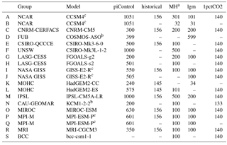
^a The name of this simulation is “midHolocene” on the Earth System Grid Federation. ^b Indicates models that only form part of PMIP3, but not CMIP5. ^c CCSM4, GISS-E2-R, and MPI-ESM-P deposited multiple ensemble members.

2.2 Observations

This research involves the joint investigation of sea surface temperature and precipitation. We adopt a combination of the twentieth century reanalysis (Compo et al., 2011) for the atmospheric variables with HadISST1.1 (Rayner et al., 2003) for the SST. HadISST1.1 forms the underlying boundary conditions for the twentieth century reanalysis (Compo et al., 2011), providing internal consistency between the datasets. These datasets exist over the period 1871–2012 CE, although there is an increased amount of uncertainty in the early portion of the record (e.g. Ilyas et al., 2017). For the mean precipitation field shown in Fig. 2, we use GPCP (Adler et al., 2003). Despite having only a shorter available record than the reanalysis, it looks to give better rainfall over the elevated topography of South America. We follow Solomon et al. (2007) in using a climatological period of 1971–2000, as the historical simulations only extend until 2005.

2.3 Definition of modes

Climate modes of variability are preferred spatial patterns associated with time variations that have global to regional impacts. Both modes of tropical Atlantic variability analysed here have been identified using area-averaged SST anomaly indices. We avoid using definitions based upon empirical orthogonal functions (EOFs) as preliminary analysis indicated they could have alternate ordering in the various models and simulations.

PMIP4 is endeavouring to perform a routine evaluation of the simulated climate variability (Kageyama et al., 2018) using the ESMValTool software (Eyring et al., 2016). This includes a collection of standardized analyses to look at coupled climate modes (Phillips et al., 2014). In particular, this research was performed using the Climate Variability Diagnostics Package (CVDP v5.0.0). We have expanded the software to additionally incorporate analysis of the predominant modes of tropical Atlantic climate variability (TAV) listed below. The main source code is freely available at http://www.cesm.ucar.edu/working_groups/CVC/cvdp/; last access: 29 August 2018. The full results of the software on the simulations described here are visible via the PMIP variability database currently hosted at http://www2.geog.ucl.ac.uk/~ucfaccb/PMIPVarData/; last access: 29 August 2018. A summary table for the climate modes mentioned here is provided as the Supplement to this article.

2.3.1 Atlantic zonal mode – ATL3

The Atlantic zonal mode (Zebiak, 1993) is the second mode of tropical Atlantic variability and represents changes in the cold tongue at the eastern part of the basin, just south of the Equator. We adopt the ATL3 region of Zebiak (1993) as a metric. It is defined to be the area average of the detrended SST anomaly over the region 3^∘ N–3^∘ S, 20–0^∘ W. This index definition is somewhat analogous to that of a Niño region in the Pacific, leading to this mode sometimes being termed the “Atlantic Niño” (Tokinaga and Xie, 2011; Xie and Carton, 2004).

2.3.2 Atlantic meridional mode – AMM

The AMM is the leading mode of variability in the Atlantic. It represents variations in the north–south SST gradient that exhibits opposite SST anomalies on either side of the mean position of the ITCZ (Servain et al., 1999). The underlying SST distribution has an influence on the position of the ITCZ, which in turn affects the regional rainfall distribution. Here we adapt the SST-based index of Doi et al. (2009). The AMM state is defined as the basin-wide, area average, detrended SST anomaly difference between the two hemispheres. More precisely, it is the average of 15–5^∘ N, 50–20^∘ W minus the average of 15^∘ S–5^∘ N, 20^∘ W–10^∘ E.

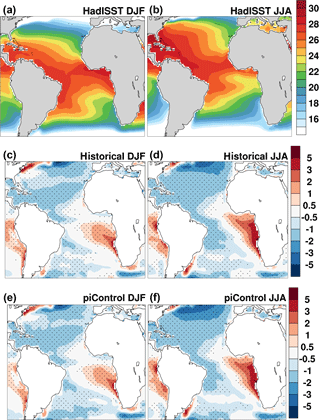
Figure 1 The sea surface temperature representation and changes in the ensemble. The climatological (1971–2000) sea surface temperature seen in HadISST (Rayner et al., 2003) for DJF (a) and JJA (b). Even on the ensemble mean, there are model biases in the seasonal temperatures of the historical simulation for DJF (c) and JJA (d). The ensemble mean biases in the seasonal temperatures in the PI control simulations for DJF (e) and JJA (f) are very similar to those of the historical simulations. Stippling indicates regions where two-thirds or more of the models agree with the sign of the ensemble mean bias (Sect. 2).

3 Present day

3.1 Mean state

Prior to investigating the inter-annual variability, it will be instructive to look at the representation of the mean climate state. The highest temperatures in the Atlantic occur on the Equator throughout the year (Fig. 1). The west Atlantic warm pool shifts to stay in the summer hemisphere. The eastern equatorial Atlantic has a tongue of cold upwelling that peaks in JJA. The warmest SSTs are associated with the strong precipitation of the ITCZ (Fig. 2). Both South America and West Africa experience heavy monsoonal rainfall in their respective summers.

General circulation models provide our best tool for modelling the climate and generally provide a fair representation. However, all models have some biases in their mean climate state. On the ensemble mean, models are unable to simulate the correct magnitude of equatorial upwelling (Fig. 1c, d). Furthermore, the west Atlantic warm pool extent is underestimated. Both of these biases are also seen for the PI control ensemble mean simulations (Fig. 1e, f) and persist throughout the year. There are precipitation biases as well (Fig. 2). In general, the models are unable to realistically represent the distribution of the ITCZ-related rainfall; there is too much rainfall on the southern flank of the ITCZ. The West African monsoon is biased dry, whilst the models have too much rainfall over NE Brazil, likely due to issues with the simulated convection. The ensemble mean biases discussed are relatively consistent within the ensemble (the majority of the biases demonstrated in Figs. 1 and 2 are stippled, meaning that two-thirds or more of the models have the same sign bias as plotted). These biases have been reported by other studies that looked at TAV in CMIP models (Breugem et al., 2006; Siongco et al., 2015; Richter et al., 2014; Deppenmeier et al., 2016; Wang et al., 2017). The bias in many of the models is related to either a weak eastern equatorial cold tongue or failure to reproduce it. Breugem et al. (2006) examine twentieth century simulations in nine GCMs and identify strong interactions between the Atlantic zonal and the meridional modes that are not realistic. They discuss the fact that the models that seem to best represent the meridional mode show its weakening in future climate conditions. Siongco et al. (2015) examined precipitation from 22 atmosphere-only models and identify an annual mean east–west bias associated with the ITCZ. They find that models with the east Atlantic bias tend to be high-resolution models which rain excessively over the Gulf of Guinea. Richter et al. (2014) analyse the simulation results of 33 models, of which 29 display biases relative to the mean state that can include an annual mean zonal equatorial SST gradient whose sign is opposite to observations. Deppenmeier et al. (2016) compare the pre-industrial simulation results of 36 different models and show that although there are errors in the annual cycles of SST, wind stress, and heat content, the relationship between them is well simulated. More recently, Wang et al. (2017) consider the validity of eastern equatorial Atlantic upwelling in the CMIP5 models when discussing their ability to predict the cold tongue SST development. Despite the mean state biases reported, the models are able to reproduce the dominant modes of climate variability in the tropical Atlantic.

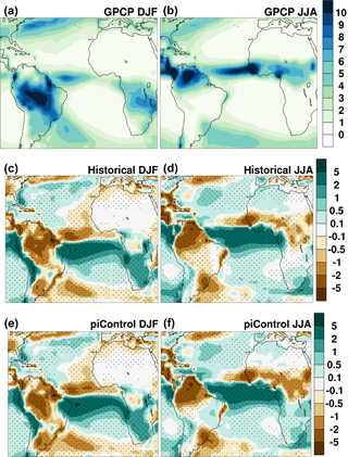
Figure 2 The seasonal cycle of precipitation and its changes across the ensemble. The climatological (1979–1999) precipitation seen in the Global Precipitation Climatology Project (Adler et al., 2003) in DJF (a) and JJA (b). The ensemble mean biases of the seasonal precipitation in the historical simulation for DJF (c) and JJA (d). The ensemble mean biases of the seasonal precipitation in the PI control simulation for DJF (e) and JJA (f). Stippling indicates regions where two-thirds or more of the models agree with the sign of the ensemble mean bias.

3.2 Representation of tropical Atlantic variability and its relationship to precipitation

To address the question of how AMM and ATL3 are simulated, we present a comparison between the ensemble mean pattern seen in the historical and PI control simulations (Table 1) together with the HadISST temperature observations (Fig. 3). The time series for both modes are determined through area-averaged, detrended SST anomalies for both the AMM (Sect. 2.3.2) and ATL3 (Sect. 2.3.1). The standard deviations of the resulting monthly time series are calculated and shown in each panel (Fig. 3). The amplitude variations of the ATL3 region are 0.18 ^∘C, which is approximately identical to the ensemble mean amplitude of 0.17 and 0.16 ^∘C (given the ensemble spread) for the historical and PI control simulations, respectively. The standard deviation SST gradient used as a metric for the AMM has a stronger amplitude in the observations (0.28 ^∘C) than the models suggest (0.18 and 0.19 ^∘C in the historical and pre-industrial, respectively). It should be noted that one should expect the GCMs to sample different phases of the low-frequency natural variability, so a direct comparison of the time series is not appropriate. Additionally, there are uncertainties in the observational record, which may be considerable in the early portion of the record (Rayner et al., 2003; Compo et al., 2011; Ilyas et al., 2017).

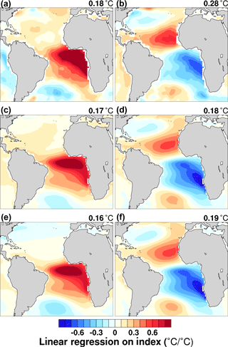
Figure 3 Sea surface temperature patterns related to ATL3 (left) and AMM (right) indices in observations (a, b) and CMIP5/PMIP3 ensemble average for the historical simulations (c, d) and the pre-industrial control (e, f). The standard deviations of the SST indices are also shown.

The spatial patterns associated with the tropical Atlantic variability are demonstrated through simple linear regression of the area-averaged indices onto the monthly anomalies (Sect. 2). This regression is extended across the globe, which highlights correlations with other modes of internal variability. This does not imply that a causal relationship extending out of the Atlantic to other ocean basins exists. The relationship with ENSO differs between models, which is interesting. However, given this model dependence, we leave analysis of this feature for future work.

The spatial extent of the ATL3 does not extend far beyond the tropical Atlantic (Fig. 3). In fact, in both observations and models it has little effect on the North Atlantic. The projection of the ATL3 in models is predominantly onto the Equator itself and there is a muted effect on the upwelling region. This is likely due to an under-representation of the upwelling in the model as demonstrated by the substantial warm biases in the mean state (Fig. 1).

The SST pattern associated with the AMM in the GCM ensembles appears to be generally well represented in the Atlantic when compared to the HadISST dataset (Fig. 3). There is too much extension of the negative SSTs across the South Atlantic, however.

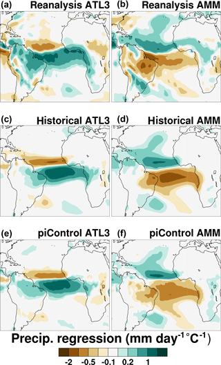
Figure 4 Precipitation patterns related to ATL3 (left) and AMM (right) indices in reanalysis (top) and CMIP5/PMIP3. The patterns across the historical simulations (c, d) and pre-industrial simulations (e, f) are an ensemble mean across the available models (Table 1).

To evaluate the relationship of the TAV modes with tropical rainfall across the region, the ATL3 and AMM indices are regressed onto precipitation for the ensemble mean historical and PI control simulations and compared to the equivalent regressions from the reanalysis. The resulting patterns are shown for two ensembles of simulations and the reanalysis (Fig. 4). It is clear from Fig. 4 that the AMM and ATL3 rainfall patterns for the simulations closely resemble that of the reanalysis. Differences are seen mostly over the continents where the relationship with the TAV modes are stronger (towards the west for South America and east–south-east for Africa). The weaker regression relationships in West Africa in the model happen to correspond to the low bias in the mean precipitation.

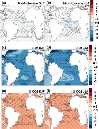
Figure 5 The climatological sea surface temperature changes shown by the ensemble. The ensemble mean difference between the mid-Holocene and pre-industrial simulations demonstrates the temperature impacts in DJF (a) and JJA (b). The Last Glacial Maximum is simulated as being substantially colder than the pre-industrial in both DJF (c) and JJA (d). In contrast, the ensemble mean average of the final 40 years of the 1 % per year increasing carbon dioxide concentration run is warmer than pre-industrial in both DJF (e) and JJA (f). Stippling indicates regions where two-thirds or more of the models agree with the sign of the ensemble mean change. Overlaid contour lines represent the mean state in the ensemble mean of the pre-industrial control simulations.

4 Past climates

4.1 Mid-Holocene

Around 6000 years ago was the warmest portion of the Holocene (Marcott et al., 2013), although there are suggestions this may only represent the summer rather than annual average temperatures (Liu et al., 2014). The magnitude of the simulated temperature changes relative to pre-industrial conditions were comparatively small (Fig. 5a, b), with several areas of cooling on the Equator (Braconnot et al., 2007). The climate change was caused by differences in the orbital precession that drove the movement of the ITCZ seasonal cycle to favour the Northern Hemisphere (Braconnot et al., 2007). Most notably, this increased the mean precipitation over Northern Africa, influencing its variability (Zhao et al., 2007) and supporting green vegetation in the Sahara (Hély et al., 2014). The ensemble simulates a noticeable northward shift in precipitation over Africa (Fig. 6b). This is, however, significantly less than observed in the region for the mid-Holocene (Perez-Sanz et al., 2014). It has been shown that, when imposing mid-Holocene vegetation reconstruction as a boundary condition to the model, inter-annual climate variability can be impacted (Pausata et al., 2017). Over NE Brazil, the monsoon rainfall reductions are relatively moderate (Fig. 6b), although there is a general decrease in summer rainfall across South America (Fig. 6a).

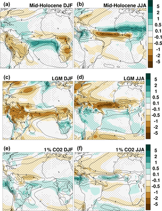
Figure 6 The changes in the seasonal cycle in precipitation across the ensemble. The ensemble mean difference between the mid-Holocene and pre-industrial simulations shows the movement of the ITCZ in DJF (a) and JJA (b). The Last Glacial Maximum is simulated as having less intense rain bands than the pre-industrial in both DJF (g) and JJA (h). In contrast, the ensemble mean average of the final 40 years of the 1 % per year increasing carbon dioxide concentration run demonstrates more enhanced activity over the ITCZ than in the pre-industrial for both DJF (i) and JJA (j). Stippling indicates regions where two-thirds or more of the models agree with the sign of the ensemble mean change. Overlaid contour lines represent the ensemble mean of the pre-industrial control simulations.

The precession-related changes in the mid-Holocene led to changes in the amplitude of TAV in many of the ensemble members (Fig. 7). These changes rarely exceed a 20 % change in amplitude. The ensemble is equivocal about the response of the ATL3 during the mid-Holocene. The ensemble mean change of 1.3 % is heavily influenced by the dramatic changes seen in KCM1-2-2 (Fig. 7). More than two-thirds of the simulations show a reduction in amplitude of the AMM (Fig. 7c), with a mean reduction of 7.5 %.

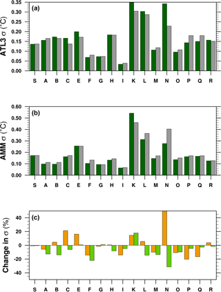
Figure 7 The standard deviations of the (a) ATL3 and (b) AMM indices in the mid-Holocene (green) and pre-industrial results (grey); (c) changes expressed as a percentage across the ensemble for both ATL3 (yellow) and AMM (light green).

There are some small local spatial patterns associated with TAV shift at the mid-Holocene (Fig. 8). The ATL3 shows hints of a northward shift in its spatial pattern (Fig. 8a). A mid-Holocene weakening of the El Niño–Southern Oscillation has been seen in observations and models (Clement et al., 2000; Chiang, 2009; Cobb et al., 2013). Despite this, there is a stronger relationship hinted at between the AMM and this mode (as seen by the increasing regressions in the Pacific in Fig. 8b). The relationships between AMM, ATL3, and ENSO are model dependent (Sect. 2), so were not investigated. The amplitude and correlations for each simulation are included as a Supplement table should subsequent researchers be interested in the links for specific models. The mid-Holocene AMM sees a poleward shift in its pattern over the North Atlantic, which is likely related to the shift in the ITCZ location in the mean state (Fig. 6a, b). There appears to be little change in the precipitation patterns associated with TAV over the continents (Fig. 8c, d). Again we must stress that the patterns shown are the ensemble mean and may average out some substantial variation in response between the individual models.

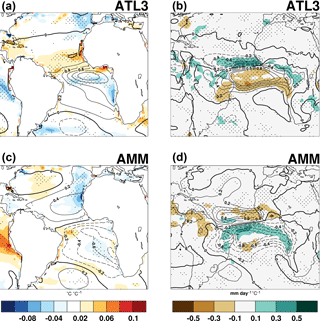
Figure 8 Mid-Holocene changes relative to pre-industrial in the temperature patterns related to (a) the ATL3 and (b) AMM indices. The changes in precipitation patterns are also shown for the ATL3 (c) and AMM (b). The changes are stippled with greater than two-thirds of the ensemble showing the same direction as the ensemble mean change. The contours show the change in regression strength onto the index in question, i.e. the change in local expression of the +1 ^∘C index. The overlaid contours show the ensemble mean strength of the relationship in the pre-industrial control. Note that the temperature regression contours are linearly spaced.

4.2 Last Glacial Maximum

21 000 years ago saw the maximum extent of the ice sheets during the last glacial. The orbital configuration then differed only slightly from the pre-industrial. The large ice sheets were accompanied by substantial cooling across the globe (Broccoli and Manabe, 1987; Clark et al., 2009; Annan and Hargreaves, 2013). Tropical sea surface temperatures cooled by roughly 2 ^∘C (Fig. 5), predominantly controlled by a drop in CO₂ of around 100 ppm (Broccoli, 2000; Marcott et al., 2014; Annan and Hargreaves, 2015).

The patterns of SST change are approximately uniform, although there is a slight weakening of the north–south gradient in the tropical Atlantic (Fig. 5). The ensemble is equivocal about changes in the equatorial zonal SST gradient. The intensity of tropical rainfall was generally reduced and the position of the ITCZ moved marginally southward (Fig. 6). The ensemble shows a strong propensity for increased climate variability in the tropical Atlantic (Fig. 9). The average increase in the ATL3 amplitude is 25.5 %, with only one dissenter suggesting a decrease. All but two models show an increasing amplitude of the AMM, with the ensemble mean increase being 31.3 % (Fig. 9).

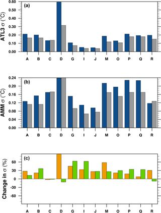
Figure 9 The standard deviations of (a) the ATL3 and (b) AMM indices in the Last Glacial Maximum simulations (blue) shown alongside the values from their respective pre-industrial control simulation (grey); (c) changes expressed as a percentage across the ensemble for both ATL3 (yellow) and AMM (light green).

These increases in amplitude are associated with small but robust changes in the spatial pattern of the modes (Fig. 10). The Last Glacial Maximum sees a slight reduction in the influence of the ATL3 in the equatorial Atlantic (Fig. 10). We interpret that to represent the ATL3 further constricting onto the Equator as the ITCZ moves slightly southward (Fig. 6). The AMM sees an increasing influence over the South Atlantic (Fig. 10b). The North Atlantic has something similar, but likely overlaid with changes caused by the imposition of large ice sheets over North America impacting the atmospheric dynamics (Pausata et al., 2011). The impact of TAV on rainfall in South America is reduced, in places by 50 % (Fig. 10c, d). These TAV-related reductions are proportionally much larger that the LGM change in mean precipitation (Fig. 6). Therefore, PMIP3 potentially suggests rainfall over NE Brazil that was simultaneously weaker, but less variable. There are few changes in the TAV patterns over Africa (Fig. 10c, d).

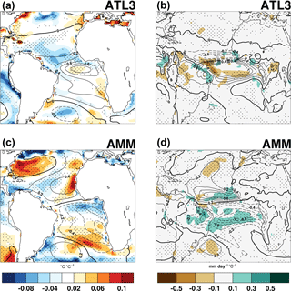
Figure 10 Last Glacial Maximum changes relative to pre-industrial in the temperature patterns related to (a) the ATL3 and (b) AMM indices. The changes in precipitation patterns are also shown for the ATL3 (c) and AMM (b). The changes are stippled with greater than two-thirds of the ensemble showing the same direction as the ensemble mean change. The contours show the change in regression strength onto the index in question, i.e. the change in local expression of the +1 ^∘C index. The overlaid contours show the ensemble mean strength of the relationship in the pre-industrial control. Note that the temperature regression contours are linearly spaced.

4.3 Future changes

The climate simulated for both the mid-Holocene (Sect. 4.1) and Last Glacial Maximum (Sect. 4.2) represent equilibrated conditions between the climate and its forcing. The climate is expected to still be in a transient state throughout the coming century. Rather than selecting a particular plausible future scenario, we analyse the idealized simulations in which the atmospheric CO₂ concentrations are increased by 1 % per year until it is quadrupled (Taylor et al., 2011). The mean climate during the final 40 years of these simulations is substantially warmer (Fig. 5) with an intensified hydrological cycle (Fig. 6). To have sufficient years to assemble robust SST patterns of climate variability, we consider the full length of these transient simulations as having first removed a linear trend from each model grid point (after Phillips et al., 2014).

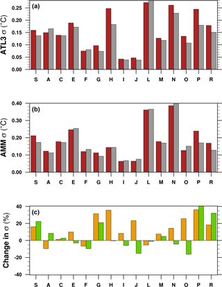
Figure 11 The standard deviations of (a) the ATL3 and (b) AMM indices in the 1 % per year until quadrupled CO₂ experiment (red) shown alongside the values from their respective pre-industrial control simulation (grey); (c) changes expressed as a percentage across the ensemble for both ATL3 (yellow) and AMM (light green).

The mean SST and rainfall patterns are very similar to a reverse of those for the cold LGM (Figs. 5, 6). However, the changes in tropical Atlantic variability are not. There is an indication that there will be an increase in amplitude of ATL3 (Fig. 11a), with an average increase of 13.8 %. However, the ensemble is split evenly as to whether the AMM (Fig. 11b) will increase in amplitude as well (mean change of +5.1 %). Despite that, there is a robust poleward expansion of the AMM influence in the Atlantic (Fig. 12b). The influence of ATL3 also expands polewards, but only in the Northern Hemisphere (Fig. 12a). Kucharski et al. (2011) demonstrate that the Pacific Ocean response to Atlantic warming is a La Niña-like cooling response, much like the AMM-related future changes in Fig. 12b. Interestingly, the precipitation response to the ATL3 is weaker in the future scenarios (Fig. 12c), with a slight contraction onto the Equator. This does not bear a strong relationship to the changes in the mean state (Fig. 6). The AMM shows a similar contraction in related rainfall, but the amplitude of the changes is generally small (Fig. 12d).

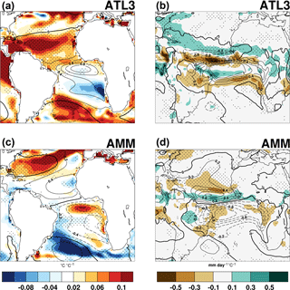
Figure 12 The 1 % per year until quadrupled CO₂ forced changes relative to pre-industrial in the temperature patterns related to (a) the ATL3 and (b) AMM indices. The changes in precipitation patterns are also shown for the ATL3 (c) and AMM (b). The changes are stippled with greater than two-thirds of the ensemble showing the same direction as the ensemble mean change. The contours show the change in regression strength onto the index in question, i.e. the change in local expression of the +1 ^∘C index. The overlaid contours show the ensemble mean strength of the relationship in the pre-industrial control. Note that the temperature regression contours are linearly spaced.

5 TAV amplitude changes as a function of the SST gradient

Changes in the amplitude of the ATL3 mode have previously been linked to changes in the zonal SST gradient since 1950 (Tokinaga and Xie, 2011). In Fig. 13, we investigate whether this link holds across the ensemble and multiple climates. We use the difference in the area-averaged SST between 3^∘ N–3^∘ S, 45–25^∘ W and 3^∘ N–3^∘ S, 20–0^∘ W to characterize the west–east SST gradient (after Tokinaga and Xie, 2011) and only consider the climate change signal to prevent the model biases from hiding any relationship. The gradient changes in the future simulations are only analysed over the final 40 years (once the main climate change signal is dominant), unlike the TAV calculations, which detrend and use the full time series (Sect. 4.3).

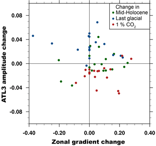
Figure 13 The change in the standard deviation of the zonal mode (ALT3) as a function of the change in the west–east SST gradient. The gradient is calculated using the Tokinaga and Xie (2011) regions (see text). The colours indicate the different experiments: 1pctCO2 (red), mid-Holocene (green), and Last Glacial Maximum (blue).

Despite the ensemble showing robust changes in mean state and often robust changes in variability, there is no apparent relationship emerging between the change in the standard deviation of the ATL3 and changes in the zonal SST gradient (Fig. 13). This perhaps questions the previous conclusions of Tokinaga and Xie (2011). In fact, extending their time series of ATL3 earlier within the instrumental period indicates little persistence of the trends they find between 1950 and 2000 (not shown). Tokinaga and Xie (2011) highlight aerosols as the cause of their trends – something which is not really explored across these simulations – leading us to conclude that further work is required to understand the future of the ATL3.

The AMM is defined as variations in the inter-hemispheric tropical SST gradient (Sect. 2.3.2). It would seem logical to think that as the inter-hemispheric gradient changes the inter-annual variability of that gradient would also change. Recently Rehfeld et al. (2018) have suggested there was an increased climate variability during the last glacial, which is well supported by Fig. 9. They propose that the increased meridional temperature gradients are the underlying cause of the greater variability. We explore this suggestion to search for an emergent constraint of the future AMM response. There appears to be no robust relationship between the AMM amplitude and the mean meridional gradient (Fig. 14). A decrease in the AMM amplitude change can be associated with an increase in the meridional SST gradient for the mid-Holocene, while the opposite occurs for the 1 % per year until quadrupled CO₂ (1pctCO2). Overall, the relationship between the amplitude change of the AMM and the changes in the meridional SST gradient depends on the climatic period considered.

6 Conclusions

This study has used the multi-model CMIP5/PMIP3 ensemble to investigate changes in tropical Atlantic variability across several climate states. All models are able to represent the main characteristics of the dominant modes of variability, with similar mean state bias, for all climate periods analysed. These biases are consistent among all models (Fig. 1), especially in the equatorial cold tongue. They are also consistent in showing precipitation biases over South America, Africa, and over the tropical Atlantic. Despite their mean state biases, the simulation results show reasonable representation of the observed patterns of tropical Atlantic variability. Analysis of the idealized warming scenarios alone suggests a spectrum of future climate change responses. The additional analysis of the palaeoclimate simulations provides some valuable context for those responses. For example, the simulated future ATL3 (Atlantic Niño) amplitude increase is not simply a response to the warmer temperatures, as a similar increase is seen during the Last Glacial Maximum.

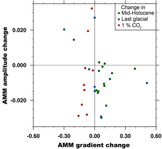
Figure 14 The change in the standard deviation of the meridional mode (AMM) as a function of the change in the meridional SST gradient. The gradient is calculated using the same regions as for the AMM index itself (Sect. 2.3.2). The colours indicate the different experiments: 1pctCO2(red), mid-Holocene (green), and Last Glacial Maximum (blue).

The spatial patterns associated with each of the tropical modes are very robust and closely related to the SST anomalies. Mode shifts actually reflect changes in intensity and amplitude rather than changes in spatial distribution. Results have shown that for the AMM behaviour in particular, the distinction between climatic periods is clear. The LGM and mid-Holocene AMM show opposite behaviour: at the LGM there is an increase in the AMM amplitude and the north–south SST gradient decreases, while at the mid-Holocene there is an increase in the north–south SST gradient accompanied by a decrease in the amplitude of the AMM. The behaviour of the AMM for the 1pctCO2 shows an overall weakening of the AMM with a decrease in both the AMM amplitude and the associated north–south SST gradient.

The study of past climate change to place future changes in context is itself worthwhile (Pancost, 2017). The advantage of using models is that they can be equally applied to the past and future (as shown here). Ideally one could use observations of past climates to constrain future projections (Hargreaves et al., 2012). Unfortunately there are currently no reconstructions of past tropical Atlantic variability to form that constraint. An alternate approach would be to detect an emergent relationship between the mean state and climate variability. Reconstructions of changes in the mean state could then be used as emergent constraints on future behaviour (Hall and Qu, 2006). We investigate whether there are such quantifiable links between TAV and the mean state in CMIP5/PMIP3: no significant relationships emerge. Nonetheless, we feel the approach of analysing several different multi-model climate experiments, some with direct or proxy observations available, promises to constrain the uncertainty in future projections.